Build
5.1 Introduction
The Build module takes data and background knowledge and outputs a set of causal models that entail the same set of conditional independence relations among the measured variables and that are compatible with any user-entered background knowledge. Build can be used to examine the class of alternatives to a given model, to locate causal regressors, to help specify causal structure, to detect the existence of latent common causes, to find "small" sets of predictors, and for other purposes.
Build works best in any of the following situations:
1. The variables are all approximately continuous and the correct model is approximately linear and multivariate normal.[1]
2. The variables are all discrete.
3. The model is neither multivariate normal nor discrete, but the user can supply the program with information about which pairs of variables are independent conditional on which other sets of variables.
If it is assumed that the correct model is linear, we suggest using the Build command to construct a set of models and then use a package such as EQS, LISREL, or CALIS to estimate the parameters and test the models suggested.[2] Chapter 14 describes the STATwriter module, which automatically creates input files for either EQS, LISREL, or CALIS.
If the variables are all discrete, then one of the models in the set output by Build can be input to the Estimate module, which will produce a maximum likelihood estimate of the parameters of this model. We describe such a procedure in section 9 of this chapter. The Estimate module is described in chapter 6.
5.2 The Input and Output of Build
Input
The simplest of Build's algorithms are described briefly in Appendix B, and are documented completely in Spirtes, Glymour, & Scheines (1993). The algorithms use statistical tests to make judgments about conditional independence relations in the population, and then use these conditional independence judgments to construct a set of causal models that entail the same set of conditional independence relations and that are compatible with any user-entered background knowledge.
In the multivariate normal case, a zero (partial) correlation is equivalent to (conditional) independence, that is, rxy.c = 0 Û x || y | c. So if raw continuous data or covariance data are entered, Build converts these data into a correlation matrix and performs a hypothesis test in which the null hypothesis is a zero partial correlation (Fig. 5.1).[3]

Fig. 5.1: Statistical tests for Structural Equation Models
If the variables are discrete, then Build tests for conditional independence with a G2 test (asymptotically distributed as c2 for contingency tables). This test is described in detail in Bishop, Fienberg, and Holland (1975) and described briefly in Appendix A.

Fig. 5.2: Statistical tests for Bayes Network
The procedures for inputting covariance matrices, cell counts, raw data (both continuous and discrete), and conditional independence facts are described in chapter 4. Inputting background knowledge is discussed later in this chapter as well in chapter 4.
Output
The output from Build is not a single causal model, but rather a set of models. What sort of output we use to represent this set depends on the assumptions you make. Besides background knowledge, which you can enter in the /Knowledge section, and general confidence in the distributional assumptions and sample, Build requires you to choose between two kinds of assumptions about latent variables.
In a given causal structure represented by DAG G, a variable z is a common cause of variables x and y if and only if in G there is a directed path from z to y and a directed path from z to x that intersect only at z. For example, in Fig. 5.3, e is a common cause of b and c. We say that a set of random variables O is causally sufficient if and only if every common cause of a pair of variables in O is itself in O. (See chapter 2 for more details about causal sufficiency.) In Fig. 5.3 the set of variables {b, c, e, f} is causally sufficient because a and d, which are left out, are not common causes of any pair in the set, but the set {a, b, c, d, f} is not causally sufficient because e is a common cause of b and c, but is not in the set.
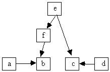
Fig. 5.3
If you assume that the variables for which you enter data are causally sufficient then the output is a pattern. If you do not assume that the variables for which you enter data are causally sufficient, then the output is a partially oriented inducing path graph, or POIPG for short.
If the population distribution satisfies the Markov and Faithfulness Conditions for the causal graph that generated it, the causal graph is acyclic, and the user-entered background knowledge is correct, then given correct statistical decisions about independence and conditional independence in the population, the causal graph that generated the data will be in the set of causal graphs represented by the output of Build, and entail the same conditional independence relations as all of the other causal graphs represented by the output of Build. (See chap. 5 of Spirtes, Glymour, & Scheines, 1993 for details.)
5.3 Using Build Assuming Causal Sufficiency
We begin with an illustration of the simplest way to use Build. We use the input file "build.dat" in Fig. 5.4.
################ build.dat ##################
/Covariance
2000
x1 x2 x3 x4 x5 x6
0.96117
1.32526 2.84005
1.39964 1.94920 3.08666
2.40187 4.24272 4.41346
8.59710
1.80106 3.19151 3.31534
6.45731 5.85505
1.73637 3.03574 3.17827
6.18110 5.62529 6.47963
################ build.dat ##################
Fig. 5.4
The following is the transcript of
a session in which we assume causal sufficiency.
Session
5.1: Using the Build Command
***************************************************
>input
Input File: build.dat
Converting covariance
matrix to correlation matrix.
>build
Output file: build.out
Assume latent common
causes? [NO]: <CR>
Test the assumption of no
latent variables? [NO]: <CR>
>exit
C:\TETRAD\RELEASE>
***************************************************
The output file produced is given in Fig. 5.5:
############ build.out ############
Output file: build.out
Data file: build.dat
Parameters:
Sample Size: 2000
Continuous Data
Covariance Matrix
x1 x2 x3 x4 x5 x6
0.9612
1.3252 2.8400
1.3996 1.9492 3.0867
2.4019 4.2427 4.4134
8.5971
1.8010 3.1915 3.3153
6.4573 5.8550
1.7364 3.0357 3.1783
6.1811 5.6253 6.4796
Significance: 0.0500
Settime: Unbounded
------------------------------------------------------
List of vanishing
(partial) correlations that made
TETRAD remove adjacencies.
Corr. : Sample (Partial)
Correlation
Prob. : Probability that
the absolute value of the sample
(partial) correlation exceeds the observed value,
on the assumption of zero (partial) correlation in
the population, assuming a
multinormal distribution.
Edge
(Partial)
Removed
Correlation
Corr. Prob.
-------
-----------
----- -----
x2 -- x3
rho(x2 x3 . x1)
0.0188 0.4015
x1 -- x6
rho(x1 x6 . x4)
0.0123 0.5820
x2
-- x6 rho(x2 x6 . x4) -0.0119 0.5954
x3
-- x6 rho(x3 x6 . x4) 0.0039 0.8597
x1
-- x5 rho(x1 x5 . x4) -0.0055 0.8043
x3
-- x5 rho(x3 x5 . x4) 0.0004 0.9852
x2
-- x5 rho(x2 x5 . x4) 0.0055 0.8047
x4
-- x6 rho(x4 x6 . x5) -0.0181 0.4187
x1
-- x4 rho(x1 x4 . x2 x3) 0.0029 0.8963
--------------------------------------------------
The Pattern (the set of
indistinguishable causal structures
under the assumption of
causal sufficiency):
x1 --- x2
x1 --- x3
x2 --> x4
x3 --> x4
x4 --> x5
x5 --> x6
############
build.out ###########
Fig. 5.5 build.out
5.4 Interpreting the Output Assuming Causal Sufficiency
All TETRAD II output files contain information about the input and output files used, and then the values of parameters relevant to the functioning of the module that produced the output. In this case the sample size, type of data, the significance level used in the statistical hypothesis tests, the covariance matrix, and the value of parameter that can control how many minutes Build is allowed to search are all printed out.
In the next section information is printed about every case in which Build made the statistical decision to accept an independence hypothesis. The Build algorithm makes the initial assumption that each pair of vertices x and y is adjacent, and then removes the adjacency between x and y whenever it finds some subset of other vertices such that x and y are independent conditional on this subset. In Fig. 5.5, for example, the first line of this section:
Edge
(Partial)
Removed
Correlation
Corr. Prob.
-------
-----------
----- -----
x2 -- x3 rho(x2 x3 . x1) 0.0188 0.4015
tells us that if the population partial correlation equals zero then the probability of observing a sample partial correlation rx2,x3.x1 with absolute value greater than .0188 is .4015. Because in this case the significance level for rejecting the null hypothesis was left at the default value of .05, this hypothesis is accepted and as a result Build removes the adjacency between x2 and x3. If the user had set the significance level higher than .4015 the hypothesis would have been rejected, and Build would not have removed the adjacency at this step in the algorithm.
Patterns
When causal sufficiency is assumed, as it is in this example, the final section of Build's output contains a pattern (Verma & Pearl, 1990) that represents a set of directed acyclic (causal) graphs that entail the same set of independence and conditional independence relations and are compatible with user-entered background knowledge. We print out a pattern because in some cases there are too many DAGs represented by the pattern to print each out individually, and because certain features common to all of the DAGs are easier to read from the pattern than from a long list of such DAGs. A very simple pattern that contains only three variables is shown below:
x1 — x2
x2 — x3
What this means is that x1 is a cause of x2 or x2 is a cause of x1, and x2 is a cause of x3 or x3 is a cause of x2, but that x1 and x3 are not both causes of x2. The pattern is a shorthand way of representing the set of DAGs shown in the following.
x1 ® x2 ® x3
x1 ¬ x2 ¬ x3
x1 ¬ x2 ® x3
but not the DAG
x1 ® x2 ¬ x3
If the directed edge x1 ® x2 appears in a pattern, then x1 ® x2 appears in every DAG represented by the pattern. In contrast if the undirected edge x1 — x2 appears in a pattern, then some of the DAGs represented by the pattern contain the edge x1 ® x2, but others contain x2 ® x1. However, although there is no constraint on the orientation of any individual undirected edge x1 — x2 in the set of DAGs represented by a pattern, there are constraints on combinations of orientations of edges in the output. We will now state the definitions more formally.
x and y are adjacent in a causal graph G iff
1) x is a direct cause of y (i.e., x is a parent of y in the causal graph) or
2) y is a direct cause of x (i.e., y is a parent of x in the causal graph).
x and y are adjacent in a pattern P iff
1) x is a direct cause of y (i.e., x is a parent of y in the pattern) or
2) y is a direct cause of x (i.e., y is a parent of x in the pattern) or
3) there is an undirected edge between x and y.
In a pattern or causal graph, if x and y both directly cause z, then we say z is a collider on any undirected path containing x ® z ¬ y. A variable is a collider on a path, however, and can be a collider on one path and a noncollider on another.
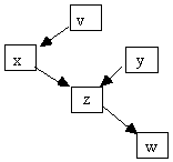
Fig. 5.6
In Fig. 5.6, for example, z is a collider on any path containing x ® z ¬ y but a noncollider on any path containing x ® z ® w.

Fig. 5.7
If x and y are not adjacent, then we say z is an unshielded collider on any undirected path containing x ® z ¬ y (Fig. 5.7). In a given pattern P, DAG G is in the set of DAGs represented by P if and only if:
1. For all vertices x1 and x2 in P, x1 and x2 are adjacent in G if and only if x1 and x2 are adjacent in P.
2. For all vertices x1 and x2 in P, if there is a directed edge x1 ® x2 in P then there is a directed edge x1 ® x2 in G.
3. For all x1, x2, x3 in P, if x1 ® x2 ¬ x3 form an unshielded collider in G then
x1 ® x2 ¬ x3 form an unshielded collider in P.
Fig. 5.8 illustrates these principles:
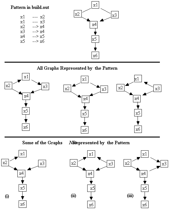
Fig. 5.8
In Fig. 5.8, the DAG labeled (i) is not a member of the set of DAGs represented by the pattern because x1 and x3 are adjacent in the pattern, but not in the DAG. (ii) is not a member of the set of DAGs represented by the pattern because the x1 — x2 and x1 — x3 edges do not form an unshielded collider in the pattern, but in the DAG the x1 ¬ x2 edge and the x1 ¬ x3 edge do form an unshielded collider. Finally, (iii) is not a member of the set of DAGs represented by the pattern because the edge connecting x3 and x4 is oriented as x3 ® x4 in the pattern, but not in the DAG.
Finding Models Equivalent to a Given Model
Whereas the output from Build is a pattern which represents an equivalence class of models, you might be interested in finding the set of models equivalent to a given model. One way to do this is to find the independence constraints entailed by this model with Monte Carlo simulation, and let Build produce a pattern that represents all the models that entail exactly these constraints. We gave such a procedure in Chap. 1, section 1.4.8. Another, less efficient alternative is to form all the graphs that have the same adjacencies as the given graph but differ as to the orientation of the adjacencies, and then remove the graphs that differ from the given graph in the set of their unshielded colliders.[4]
Estimating and Testing a Model
If the data given to the Build command are assumed to have been generated by a linear model, then any of the DAGs in the set represented by the pattern correspond to a linear recursive structural equation model in which each variable is a linear function (with undetermined coefficients) of its parents in the DAG plus an independently distributed error variable. The linear recursive structural equation model corresponding to the DAG can be estimated and tested by statistical packages such as EQS, LISREL, or CALIS. Chapter 14 describes STATwriter, a TETRAD II module for automatically constructing input files for either EQS, LISREL, or CALIS.
If the data given to Build are assumed to have been generated by a discrete Bayesian network, then any DAG represented by the pattern can be used as input to the Estimate command, which will calculate a maximum likelihood estimate of the parameters of the Bayes network. (See chapter 6 for details.) TETRAD II provides no way to test an estimated Bayesian network.
Double Headed Edges in the Pattern
The output of Build with causal sufficiency may contain bidirected, or double-headed edges, for example, x1 « x2. If the conditional independence decisions made by the algorithm are correct, the existence of a bi-directed edge x1 « x2 in a pattern suggests that there is a latent common cause of x1 and x2 (see Chap. 2, section 2.4.3 for more details) and Build should be run again on the same data without assuming causal sufficiency. (However, the Monte Carlo simulations described at the end of this chapter also indicate that the most common kind of mistake that Build makes is putting too many arrowheads into its output.)
"#" in the Pattern
If Build cannot find a consistent orientation of an edge, it places a "#" next to it in the output. This can happen if some statistical tests indicate that an edge should be oriented as x1 ® x2, and other statistical tests indicate that it should be oriented as x1 ¬ x2.
5.5 Testing the Assumption of No Latent Common Causes
If the user is constructing a linear model, and there are fewer than 15 variables in the model, Build will ask if you wish to test the assumption that there are no latent common causes (causal sufficiency). (Recall that we assume that all of the error terms in an RSEM are uncorrelated. We represent a correlated error between x and y by introducing a new latent variable Z that is a common cause of x and y. This test for latent common causes can also be viewed as a test of the assumption of uncorrelated errors.) The presence of double-headed arrows in the output is one indication that latent common causes may be present; however, there are other tests for latent common causes that can be used even if there are no double-headed arrows present. Unfortunately, the time the test requires is exponential in the number of variables. On Unix workstations such as a Decstation 3100, the test takes several minutes for about 10 variables, and more than 1/2 hour for 15 variables. The test may take even longer on the DOS version of TETRAD II.
The test of causal sufficiency is
performed in the following way. For linear models, Build uses zero partial
correlations to construct its output. There is another class of constraints,
the vanishing tetrad differences (described in chap. 2)
that can be used to test whether there are latent variables in linear models. A
vanishing tetrad difference is an equation of the form ri,jrk,l
![]() ri,krj,l
= 0, where i, j, k and l are four distinct variables. Each tetrad difference is
judged to be equal to zero in the population if that hypothesis is not rejected
by a statistical test. Each DAG entails a certain (possibly empty) set of
vanishing tetrad differences, regardless of the numerical values of the linear
coefficients or the distributions of the exogenous variables. A DAG entails
that a tetrad difference vanishes only if it also entails that certain sets of
partial correlations vanish. If a tetrad difference among four variables is
judged to vanish in the population, but the corresponding sets of partial
correlations are judged not to vanish, then the program concludes the
assumption of causal sufficiency has been violated.[5]
ri,krj,l
= 0, where i, j, k and l are four distinct variables. Each tetrad difference is
judged to be equal to zero in the population if that hypothesis is not rejected
by a statistical test. Each DAG entails a certain (possibly empty) set of
vanishing tetrad differences, regardless of the numerical values of the linear
coefficients or the distributions of the exogenous variables. A DAG entails
that a tetrad difference vanishes only if it also entails that certain sets of
partial correlations vanish. If a tetrad difference among four variables is
judged to vanish in the population, but the corresponding sets of partial
correlations are judged not to vanish, then the program concludes the
assumption of causal sufficiency has been violated.[5]
We generated a Monte Carlo sample from a randomly parameterized linear model with the causal structure shown in Fig. 5.9. We calculated the covariance matrix for all variables except for T, and formed an input file for TETRAD II called "build2.dat."
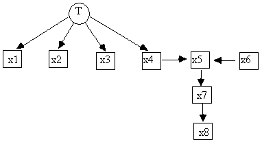
Fig. 5.9: Generating DAG for build2.dat
We then ran the Build module on this data (session 5.2), but incorrectly assumed that our input variables were causally sufficient. That is, we answer no to the question:
Assume
latent common causes? [NO]:
even though the generating model includes T, which is a common cause of several pairs of the x variables.
Session
5.2: Using the Build command
***************************************************
>input
Input File: build2.dat
Converting covariance
matrix to correlation matrix.
>build
Output file: build2.out
Assume latent common
causes? [NO]: <CR>
Test the assumption of no
latent variables? [NO]: yes
>exit
C:\TETRAD\RELEASE>
***************************************************
The relevant part of build2.out is shown in Fig. 5.10. After the pattern, tetrad equations that hold statistically but that cannot be explained without latent variables are listed.
############ build2.out
################
--------------------------------------------------
The Pattern (under the assumption of causal sufficiency):
x1 --- x2
x1 --- x3
x1 --- x4
x2 --- x3
x2 --- x4
x3 --- x4
x4 --> x5
x6 --> x5
x5 --> x7
x7 --> x8
x1
x2 x3 x4 - x1 x3 x2 x4 may need a
latent variable
x1
x4 x2 x3 - x1 x2 x3 x4 may need a
latent variable
x1
x3 x2 x4 - x1 x4 x2 x3 may need a
latent variable
x1
x2 x3 x5 - x1 x3 x2 x5 may need a
latent variable
x1
x5 x2 x3 - x1 x2 x3 x5 may need a
latent variable
x1
x3 x2 x5 - x1 x5 x2 x3 may need a
latent variable
x1
x2 x3 x7 - x1 x3 x2 x7 may need a
latent variable
x1
x7 x2 x3 - x1 x2 x3 x7 may need a
latent variable
x1
x3 x2 x7 - x1 x7 x2 x3 may need a
latent variable
x1
x2 x3 x8 - x1 x3 x2 x8 may need a
latent variable
x1
x8 x2 x3 - x1 x2 x3 x8 may need a
latent variable
x1
x3 x2 x8 - x1 x8 x2 x3 may need a
latent variable
################# build2.out
##############
Fig. 5.10
The pattern is shown as a diagram in Fig. 5.11.
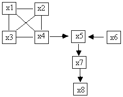
Fig. 5.11
Because the assumption of causal
sufficiency was violated for the measured variables x1-x8 by the true DAG, x1,
x2, x3, and x4 are all adjacent in the pattern. There is nothing in the output
pattern itself that indicates that the assumption was violated. However, the
first line following the output pattern indicates that the zero tetrad
difference rx1,x2rx3,x4 ![]() rx1,x3rx2,x4
is judged to hold in the population, but it is not entailed by any DAG with
just those variables that also entails exactly the zero partial correlations
judged to hold in the population. Similarly, the following lines list other
tetrad differences that are judged to hold in the population and that are not
entailed by any DAG in the set represented by the pattern. However, these zero tetrad differences may be entailed by a DAG with
latent variables that also entails the conditional independence relations
judged to hold among the measured variables, for example, the DAG in Fig.
5.9. If a given zero tetrad difference such as rx1,x2rx3,x4 - rx1,x3rx2,x4 = 0 is entailed by some DAG that
also entails the conditional independence relations judged to hold in the
population among the measured variables, then that DAG contains a latent common
cause of at least one of the two pairs x1 and x4, or x2 and x3.
rx1,x3rx2,x4
is judged to hold in the population, but it is not entailed by any DAG with
just those variables that also entails exactly the zero partial correlations
judged to hold in the population. Similarly, the following lines list other
tetrad differences that are judged to hold in the population and that are not
entailed by any DAG in the set represented by the pattern. However, these zero tetrad differences may be entailed by a DAG with
latent variables that also entails the conditional independence relations
judged to hold among the measured variables, for example, the DAG in Fig.
5.9. If a given zero tetrad difference such as rx1,x2rx3,x4 - rx1,x3rx2,x4 = 0 is entailed by some DAG that
also entails the conditional independence relations judged to hold in the
population among the measured variables, then that DAG contains a latent common
cause of at least one of the two pairs x1 and x4, or x2 and x3.
5.6 Using Build Without Assuming Causal Sufficiency
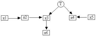
Fig. 5.12
The file build3.dat contains Monte Carlo generated covariance data on x1 - x6 from a random parameterization of a linear model with the causal DAG in Fig. 5.12. Session 5.3 shows how to use the Build command when it is not assumed that the measured variables are causally sufficient.
Session
5.3: Build without causal sufficiency
***************************************************
>input
Input File: build3.dat
>build
Output file: build3.out
Assume latent common
causes? [NO]: yes
Use the exact algorithm?
[YES]: <CR>
>exit
***************************************************
Without the assumption of causal sufficiency, the class of causal models represented by the output of Build is much larger, and thus the causal conclusions that can be drawn are much weaker. The program queries whether the user would like to use the exact algorithm, or a heuristic algorithm. The exact algorithm is sometimes much slower than the heuristic algorithm, and in many cases the two procedures give the same output. However, there are certain unusual causal structures where the exact algorithm produces the correct output (at least if it makes the correct judgments about which variables are conditionally independent) and the heuristic algorithm does not. We suggest using the heuristic algorithm if the exact algorithm takes too long. (If the exact algorithm takes too long, another alternative is to set an upper limit to how long the exact algorithm will run before aborting and reporting what it has learned in the time allotted. This is explained in section 5.7.1.) The interpretation for the output is the same regardless of whether the exact or the heuristic algorithm is used, so we will not illustrate the use of the heuristic algorithm. The relevant part of the output file build3.out is given in Fig. 5.13.
############ build3.out #############
NOT assuming causal sufficiency
The Partially Oriented Inducing Path Graph (POIPG):
x1 o-o x2
x2 o-> x3
x3 --> x6
x3 <-> x4
x5 o-> x4
Directed Paths
x3 to x6
Not Connected by Directed
Paths
x1 to x4
x1 to x5
x2 to x4
x2 to x5
x3 to x1
x3 to x2
x3 to x4
x3 to x5
x6 to x1
x6 to x2
x6 to x3
x6 to x4
x6 to x5
x4 to x1
x4 to x2
x4 to x3
x4 to x6
x4 to x5
x5 to x1
x5 to x2
x5 to x3
x5 to x6
############ build3.out #############
Fig. 5.13: build3.out
The POIPG in build3.out is shown in Fig. 5.14.

Fig. 5.14
5.6.1 Interpreting Partially Oriented
Inducing Path Graphs (POIPGs)
The output from Build without the assumption of causal sufficiency is a partially oriented inducing path graph, or POIPG. The full meaning of a POIPG is complicated, and is explained in more detail in Spirtes, Glymour, and Scheines (1993). The important information about the influence of measured variables on one another can be found by applying the following rules.
1. The first line under the heading "Directed Paths" is "x3 to x6." That indicates that x3 is a cause of x6, i.e. in the directed graph that represents the causal process that generated the data there is a directed path from x3 to x6.
2. The first line under the heading "Not Connected by Directed Paths" is "x1 to x4". This indicates that x1 is not a cause of x4, i.e. in the directed graph that represents the causal process that generated the data there is no directed path from x1 to x4.
3. An edge x3 « x4 means that there is a latent common cause of x3 and x4.
4. A "#" sign next to a pair of variables in the list of causal relations means that the program could not find a consistent orientation of the edge.
5. An edge x o® y indicates that either x is a cause of y, or there is a common latent cause of x and y, or both.
6. An edge x o-o y indicates that either x is a cause of y or y is a cause of x, or there is a common latent cause of x and y, or some combination of these.
Thus from the output in build3.out (Fig. 5.13) we can infer that x3 is a cause of x6, that x3 and x4 have an unmeasured common cause, and that x1 and x2 have no influence on x4 and x5, nor do x4 and x5 have any influence on x1 and x2.
It is important to understand that although the POIPG contains information about what paths do or do not exist in the graph that generated the POIPG, it does not in general contain much information about what variables lie along those paths. As the example in Fig. 5.15 shows, if there is a directed edge from x3 to x5 in the POIPG, although this implies that in the generating graph G there is a directed path from x3 to x5, it does not in general imply that the directed path from x3 to x5 in G contains none of the other variables in the POIPG, that is, x3 may be an indirect cause of x5 in G, relative to the variables in the POIPG, rather than a direct cause of x5.
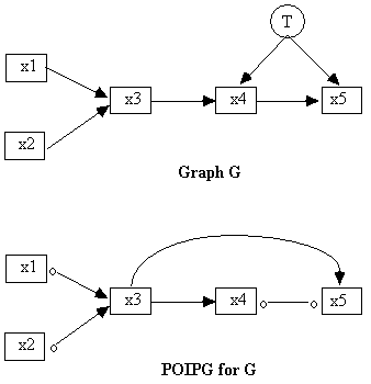
Fig. 5.15
In this case we cannot conclude from the POIPG that x3 is a direct cause of x5 relative to the set of variables in the POIPG, even though there is an edge x3 ® x5 in the POIPG. However, we can conclude that x3 is a cause (either direct or indirect) of x5 relative to the variables in the POIPG.
Similarly, although x1 « x2 in a POIPG implies that there is a latent common cause T of x1 and x2 in the generating graph G, we cannot in general tell if T is an indirect or a direct common cause of x1 and x2. That is, although we can conclude that there is some latent variable T and directed paths from T to x1 and x2 in G, those directed paths may contain other variables in the POIPG besides x1 and x2.
There is one special circumstance under which it is possible to tell from a POIPG that a variable x is a direct cause of y (that is, in the generating graph, there is a directed path from x to y that contains none of the other variables in the POIPG.) Informally, a semidirected path from x to y in a POIPG is a sequence of edges between x and y such that none of the edges has an arrowhead that points back at x. In Fig. 5.14, for example, x1 o-o x2 o® x3 is a semidirected path from x1 to x3. However, x1 o—o x2 o® x3 « x4 is not a semi-directed path from x1 to x4, because the edge between x3 and x4 contains an arrowhead pointing back towards x1. In Fig. 5.14 there is a directed edge from x3 to x6, and no other semi-directed path from x3 to x6. Under these circumstances we can conclude that x3 is a direct cause of x6.
The informativeness of the POIPG output depends on two factors:
1. The structure of the causal process that generated the data.
2. Which variables were measured.
We will illustrate the different roles that the latent variables allowed by a POIPG may play with the following example. Suppose that the output of Build is as shown in Fig. 5.16. This is very uninformative output, because each of the variables is adjacent to every other variable, and no adjacency is even partially oriented. In general, "sparse" POIPGs are much more informative than "dense" POIPGs.

Fig. 5.16
This POIPG is compatible first of all with graphs that have no latent variables at all, like the graph in Fig. 5.17 or any equivalent to it.

Fig. 5.17
It is also compatible with the latent variable graph shown in Fig. 5.18 (where this time we have explicitly included the error terms in order to make the following point). In Fig. 5.18, T1 is a latent common cause of a and b, and of a and c, and T2 is a latent common cause of b and c. b is an imperfect measure of T2 because of the presence of an unmeasured error term that also contributes to the value of b. So the structure among the latent variables T1, T2, and T3 is not reflected in any conditional independence relations among a, b, and c.[6]
In general, if you believe that the measured variables are indicators of latent variables, and the correlations between the measured variables are produced by connections among the latent variables, Build will give output that is correct, but uninformative about the latent structure. In general, forming combinations of measured variables (by averaging for example) that are intended to serve as scales also will not help. Under these circumstances, and the assumption of linearity and normality, it may be more appropriate to use Purify and MIMBuild (see chap. 9 and 10). In the discrete case we do not have any method that is informative and reliable about the latent structure.
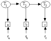
Fig. 5.18
Another graph that is compatible with the POIPG in Fig. 5.16 is shown in Fig. 5.19.
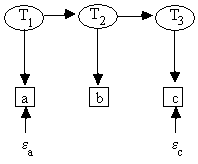
Fig. 5.19
In this case, suppose that b is an imperfect measure of T2 not because it is also caused by some
unmeasured error term, but because b "collapses" some of the
distinctions made by T2.
Suppose for example that T2
was blood pressure, as measured by two real numbers, and b was blood pressure
simply classified as "low," "normal," and "high."
So the latent variables that may be present according to the output of the
Build algorithm include latent variables that are simply more
"refined" versions of the measured variables.
In the Examples section at the end of this chapter, the Lung Capacity example shows how to use Build when causal sufficiency is not assumed.
5.7 Adding Background Knowledge and Time Limits
By adding background knowledge, you can place constraints on the model constructed by Build. You can give the program a limit on the amount of time it runs; you can specify the time order of any of the variables (so that the program will not consider the possibility that later variables cause earlier variables) and you can eliminate from consideration individual edges or common causes of specific pairs of measured variables.
5.7.1 The Settime Command
The time that the Build command takes to run depends on how many variables are in the data, and the causal structure that it constructs. In some cases the building process may take longer than you wish to wait. On the Unix version, if you wish to stop a building process that is already going on, hold the control key down while striking "\".[7] On the PC version, hold down the control key while striking "g".
The Settime command allows the user to set the maximum number of minutes used in the search conducted by the Build command. Using the settime command is simple:
/Knowledge
settime 60
Fig. 5.20
The time is measured in minutes. When a maximum amount of time is set by the user, the building process will stop when that time is exceeded, and print out the results obtained so far. When this occurs, the output, whether causal sufficiency is assumed or not, may contain too many causal connections, rather than too few. The program may take a little longer to stop than the maximum time indicated, because only some parts of the algorithms stop to check whether the time limit has been exceeded.
5.7.2 Temporal Information
The Addtemporal and Removetemporal commands are used to store temporal information about the variables. Suppose x67 and y67 were measured in 1967, x72 and y72 were measured in 1972, x84 was measured in 1984, and the temporal relationship of z1 to the other variables is not known. No model that suggests an edge from a later variable to an earlier variable should be allowed. These models can be eliminated from consideration in the model search procedure by using the Addtemporal command in the following way:
/Knowledge
addtemporal
1 x67 y67
3 x84
2 x72 y72
Fig. 5.21
Temporal information can be removed with the Removetemporal command. Details about the syntax of these commands is given in chapter 4.
5.7.3 Requiring Edges
If a user wishes to require that certain edges appear in the output of the Build command, those edges should be listed in the /Graph section of an input file. The format of the /Graph section is explained in detail in chapter 4. Build pays no attention to edges in the graph that contain latent variables.
The /Graph section serves two distinct purposes in Build. First, the /Graph section is the starting point for Build. That is, the graph input in the /Graph section is a subgraph of each graph G in the set of graphs represented by the output of each of these modules. Second, the graph allows the user to select a subset of the variables that appear in the data for use by Build; that is, the only variables that appear in the models output by Build are variables that appear in the graph. If a user wishes a variable to be included in the output of Build, but the variable is not known to be adjacent to any other variable in the graph, the user can add to the graph a line that contains just that vertex. For example, suppose that the user wishes Build to construct a model containing just the variables x1, x2, x3, x4, but the only causal dependencies that she knows in advance are that x1 directly causes x2 and x2 directly causes x3. The appropriate input graph is then shown in Fig. 5.22:
/graph
x1 x2
x2 x3
x4
Fig. 5.22
The output of the Build command is then guaranteed to contain the edges x1 to x2, and x2 to x3; in addition, the variable x4 will appear in the output of the command. x4 may or may not appear adjacent to other variables in the output, depending upon the results of the statistical tests performed by the Build command. x5 will not appear in the output, even if it occurs in the data, because it is not mentioned in the graph.
If no /Graph section is read as input, the default graph contains all of the variables mentioned in the data, but no edges. In effect, this default initial graph tells the program that Build's output should contain all of the variables mentioned in the data, but puts no constraints upon what edges appear in the set of graphs represented by the output.
5.7.4 Forbiddirect, Forbidcommon, Allowdirect, and Allowcommon
The Forbiddirect command is used to specify edges that are forbidden to appear in any model constructed by the Build command. If background knowledge indicates that x1 cannot cause x2, and x2 cannot cause x3, these restrictions can be entered in the following way:
/Knowledge
Forbiddirect
x1 x2
x2 x3
Fig. 5.23
The first line of the command states what sort of causal connection is being forbidden, a direct edge in the case illustrated, and a common cause if Forbidcommon is used. The command line Forbiddirect is followed by a list of edges, one edge per line. Each edge is specified exactly as it is in a /Graph section, that is, the cause followed by a space followed by the effect. A blank line after the x2 x3 line indicates that the Forbiddirect command is ended. The Allowdirect command acts in an analogous fashion, but undoes the effect of a Forbiddirect command.
The Forbidcommon command acts in the same way as the Forbiddirect command except that it instructs the search command not to consider a latent common cause between two variables. Similarly, the Allowcommon command undoes the effect of a Forbidcommon command. Forbidding common causes has no effect on the Build procedure when it is assumed that the true model has no latent common causes.
Note that to completely eliminate any connection between variables x1 and x2 under the assumption that there are no latent common causes of x1 and x2, you must forbid the edge x1 ® x2 and the edge x2 ® x1 (either by using the Addtemporal or the Forbiddirect commands.) To completely eliminate any connection between variables x1 and x2 without the assumption that there are no latent common causes of x1 and x2, you must not only forbid the edge x1 ® x2 and the edge x2 ® x1, you must also forbid a common cause of x1 and x2 (by using the Forbidcommon command.)
5.8 Choosing the Significance Level and
Reliability
The Build algorithm tests for vanishing partial correlations (in the linear case) or conditional independence facts (in the discrete case.) The outcomes of the these tests guide the program in deciding whether to include edges between pairs of variables. The decision to reject or not to reject the hypothesis that a partial correlation is zero depends on the significance level used in the tests. Because Build performs a complex sequence of statistical tests, each at the given significance level, the significance level is not an indication of error probabilities of the entire Build procedure. The default significance level in the program is .05, but it can be altered by typing "sig" at the TETRAD prompt and then entering the preferred value when the program responds. There is no true or correct value of the significance level; the right value to use is the one that gives the most reliable output from the program. Extensive simulation tests with random DAGs lead us to the following recommendations for the linear case:
Sample size 100 or smaller: Set the significance level at .2
Sample size 100 to 300: Set the significance level at .1
Larger samples: Use the default significance level of .05 or smaller.
These are rules of thumb. We recommend that the user vary the significance level to obtain an idea of how robust the output is. The reasons for these suggestions are that the program tends to underfit-that is to include too few edges-at small sample sizes. Increasing the significance level makes it easier for the program to retain edges between variables.
In order to test the speed and the reliability of the Build algorithm on linear models assuming causal sufficiency, we have tested it on a large number of simulated examples. The degree of a vertex in the graph is the number of vertices it is adjacent to. The average degree of the vertices in the graphs considered are 2, 3, 4, or 5; the number of variables is 50; and the sample sizes are 100, 200, 500, 1,000, 2,000, and 5,000. For each combination of these parameters, 10 graphs were randomly generated, randomly parameterized, and a single sample taken from each parameterized DAG.
All pseudo-random numbers were generated by the UNIX "random" utility. Each sample is generated in three stages:
1. The graph is pseudo-randomly generated.
2. The linear coefficients (in the linear case) or the conditional probabilities (in the discrete case) are pseudo-randomly generated.
3. A sample for the model is pseudo-randomly generated.
For simulated continuous distributions, an "error" variable was introduced for each endogenous variable and values for the linear coefficients between .1 and .9 were generated randomly from a uniform distribution for each edge in the graph. The exogenous variables-including the error terms-were generated independently from a standard normal distribution, and values of endogenous variables were computed as linear functions of their parents and an error term.
Reliability has several dimensions. A procedure may err by omitting undirected edges in the true graph or by including edges-directed or undirected-between vertices that are not adjacent in the true graph. For an edge that is not in the true graph, there is no fact of the matter about its orientation, but for edges that are in the true graph, a procedure may err by omitting an arrowhead in the true graph or by including an arrowhead not in the true graph. We call the pattern the PC algorithm would generate given the population correlations the true pattern. We call the pattern the algorithm infers from the sample data the output pattern. An edge existence error of commission (Co) occurs when any pair of variables are adjacent in the output pattern but not in the true pattern. If an edge e between x and y occurs in both the true and output patterns, there is an edge direction error of commission when e has an arrowhead at x in the output pattern but not in the true pattern (and similarly for y). Errors of omission (Om) are defined analogously in each case.
The Build procedure was run using a significance level of .05 on all trials. The graphs on the following pages show the results. Each point on the graph is a number, which represents the average degree of the vertices in the directed graphs generating the data. In each case the results are plotted separately for graphs of degree 2, 3, 4, and 5.


Fig. 5.24


Fig. 5.25
The following qualitative conclusions can be drawn.
1. The rates of arrow and edge omission decrease dramatically with sample size up to about sample size 1,000; after that the decreases are much more gradual.
2. The rates of arrow and edge commission vary much less dramatically with sample size than do the rates of arrow and edge omission.
3. As the average degree of the variables increases, the average error rates increase in a very roughly linear fashion.
4. At high average degree and low sample sizes the output of each of the procedures tends to omit over 50% of the edges in the true graph. At large sample sizes and low average degree only a few percent of the true edges are omitted, but with high average degree the percentage of edges omitted even at large sample sizes is significant.
5. Arrow commission errors are much more common than edge commission errors. If an arrow does not occur in a graph, there is a considerable probability for any of the procedures that the arrow will be output, unless the sample size is large and the true graph is of low degree.
The results suggest that the programs can reasonably be used in various ways according to the size of the problem, the questions one wants answered, and the character of the output.
In general, the procedure will be more informative, more reliable, and faster, if the actual causal structure generating the sample data is represented by a sparse DAG; a DAG in which every pair of variables is connected by an edge often indicates that the sample is a mixture of systems with different causal processes.
The Build procedure is not very reliable if most variables are binary, because spurious independencies tend to arise in such cases. Moving to as few as three values for variables makes a considerable difference in the reliability of the Build output.
To get a more specific sense for how reliable the search procedure is for a particular sample size, number and kind of variables and generating structure, we recommend using the Monte Carlo facility in the program. This is explained in more detail in chapter 13, section 6.
5.9 Examples
In chapter 1, section 1.4, we discuss seven ways to use TETRAD II to help solve common modeling problems. The solutions to the first several involve the Build module. Here we include several more examples. In the first we consider an empirical data set on gender, socioeconomic status, parental encouragement and college plans. We also use this example to illustrate the Estimate and Update modules in chapters 6 and 7. In the second example, we show how Build can be used to accurately recover almost all of a large causal model about emergency medicine. In the third example, we show how Build can obtain correct answers about direct causation where multiple regression and best subsets regression cannot.
5.9.1 College Plans
Many variables of interest are better measured by categories than by a real variable. Just as with linear models, one of the common uses of models for discrete variables is to attempt to represent and quantify causal dependencies (Fienberg, 1977). The same difficulties that beset the discovery of causal relationships among continuous variables apply in the discrete case.
Sewell and Shah (1968) studied five variables from a sample of 10,318 Wisconsin high school seniors. The variables and their values were:
sex [male = 0, female = 1]
iq = Intelligence Quotient, [lowest = 0, highest = 2]
cp = college plans [yes = 0, no = 1]
pe = parental encouragement [0 = low, 1 = high]
ses = socioeconomic status [0 = lowest, ... 3 = highest]
They offered the following sensible causal hypothesis:
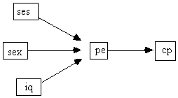
Fig. 5.26
Some questions naturally arise: do sex, iq, and socioeconomic status have any influence on college plans other than through parental encouragement? Does ses influence iq? How can the joint probabilities be estimated? How, for example, can the probability of a male child planning for college be compared with the probability of a female child planing for college?
To use Build in order to analyze the same data set, we first create an input file (shaw.dat), that contains cell counts exactly as they are given in Fienberg's (1977) account of the data. Because iq, parental encouragement and socioeconomic status cannot cause sex, and college plans cannot cause any of the other variables, we include these restrictions in a knowledge section. Session 5.4 shows how to run Build on this data.
Session 5.4: Build on data on college plans
************************
>input
Input File: shaw.dat
>build
Output file: shaw.out
Assume latent common
causes? [NO]: <CR>
>exit
************************
Notice that after we answered yes to the question about causal sufficiency, we were not prompted about whether we wanted to test this assumption with the data. That is because the data in this case are for discrete variables and the test we discussed in section 5 works for linear models.
The pattern in shaw.out is shown in Fig. 5.27:
############### shaw.out ################
The Pattern (the set of indistinguishable causal structures
under the assumption of
causal sufficiency):
sex --> pe
iq --> cp
iq --> pe
iq --- ses
pe --> cp
ses --> cp
ses --> pe
############### shaw.out ################
Fig. 5.27: Shaw.out
Fig. 5.28 shows this pattern drawn graphically.

Fig. 5.28
Build cannot orient the edge between iq and ses. As far as the program can determine, the causal connection between iq and ses might be due to an influence of ses on iq, or of iq on ses, or to an unmeasured common cause of both. It seems unlikely that the child's intelligence causes the family socioeconomic status, and the only sensible interpretation is that ses causes iq, or that they have a common unmeasured cause. Because the program will not estimate discrete models with latent variables, we assume the former. Thus we can specify a particular member of the set of indistinguishable models represented by the pattern in Fig. 5.28 with the TETRAD II input file shaw.g (Fig. 5.29).
############## shaw.g ##############
/graph
sex pe
iq cp
iq pe
ses iq
pe cp
ses cp
ses pe
############## shaw.g ##############
Fig. 5.29: shaw.g
We can now ask the program to estimate the probability distribution, and we show how in the next chapter. The resulting output contains an explicitly written probability for every value of each variable conditional on its parents, starting with the variables ses and sex that have no parents in the input DAG. Suppose now you want to compare the probabilities that male and female children, respectively, plan to go to college. This is easily done with the estimated model with TETRAD II's Update module, and we show how in chapter 7.
5.9.2 A Large Causal Model of Discrete Data
Some search procedures for models of discrete data not only have no proofs of their reliability, they run into computational problems with more than a dozen variables, or even fewer depending on how many categories each variable may have. (One exception is the algorithm described in Cooper & Herskovits, 1992, which for this example is slightly more reliable than Build given a linear temporal order. However, current implementations of their algorithm require a known time order for the variables.). The diagram in Fig. 5.30, called the ALARM network, was developed as a model of an emergency medical system (Beinlich, et al. 1989). The variables are all discrete, taking two, three, or four distinct values. In most instances a directed arrow indicates that one variable is regarded as a cause of another. The physicians who built the network also assigned it a probability distribution: Each variable V is given a probability distribution conditional on each vector of values of the variables having edges directed into V.
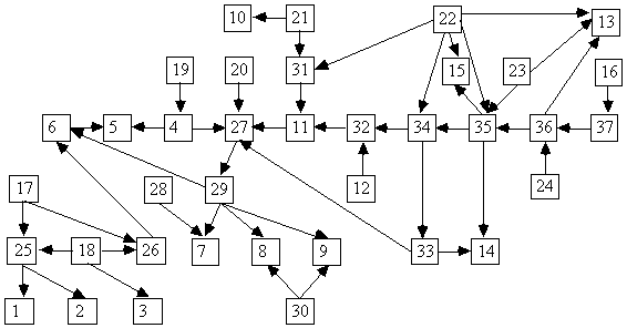
Fig. 5.30: The ALARM Belief Network
KEY:
1 - central venous pressure 20 - insufficient anesthesia or
analgesia
2 - pulmonary capillary wedge pressure 21 - pulmonary embolus
3 - history of left ventricular failure 22 - intubation status
4 - total peripheral resistance 23 - kinked ventilation tube
5 - blood pressure 24 - disconnected ventilation tube
6 - cardiac output 25 - left-ventricular end - diastolic
volume
7 - heart rate obtained from blood pressure 26 - stroke volume
monitor
8 - heart rate obtained from electrocardiogram 27 - catecholamine level
9 - heart rate obtained from oximeter 28 - error in heart rate reading due to
low cardiac output
10 - pulmonary artery pressure 29 - true heart rate
11 - arterial-blood oxygen saturation 30 - error in heart rate reading due to electrocautery device
12 - fraction of oxygen in inspired gas
13 - ventilation pressure 31 - shunt
14 - carbon-dioxide content of expired gas 32 - pulmonary-artery oxygen
saturation
15 - minute volume, measured 33 - arterial carbon-dioxide content
16 - minute volume, calculated 34 - alveolar ventilation
17 - hypovolemia 35 - pulmonary ventilation
18 - left-ventricular failure 36 - ventilation measured at
endotracheal tube
19 - anaphylaxis 37 - minute ventilation measured at
the ventilator
Fig. 5.30
The DAG has 37 variables and 46 edges. Another group of computer scientist/physicians .;(Herskovits & Cooper, 1990) used the diagram to generate simulated emergency medicine statistics for 20,000 individuals. The data is in alarm.dat. From half or even a tenth of the data, Build's output (a pattern) includes almost all of the adjacencies ALARM network, and has information about the directions of most of the edges. Depending on sample size, the program makes two or three errors in identifying adjacencies and four or five errors in determining the directions of influence.
5.9.3 Regression and Build
To illustrate the advantages of Build over regression, consider the following problem. Suppose that the unknown true causal structure is shown in Fig. 5.31 and that each variable is a linear function of its parents in the graph and an independent error term. x1 through x5 and y are measured, while T is latent. The goal is to find which of the x variables is a direct cause of y relative to {x1, x2, x3, x4, x5, y}, given the marginal distribution. In large samples, for data from this structure, linear multiple regression will give all variables in the set {x1, x2, x3, x5} nonzero regression coefficients, even though neither x2 nor x3 has a direct influence on y. A variety of best subsets regressions give similar results. If a specification search for regressors had selected only x1, or x1 and x5, a regression on these variables would give consistent, unbiased estimates of their direct influence on y. But the textbook procedures in commercial statistical packages will in all of these cases fail to identify {x1} or {x1, x5} as the appropriate subset of regressors.
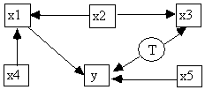
Fig. 5.31
In contrast, if the marginal distribution is given to the Build module, and causal sufficiency is not assumed, Build produces the following POIPG as output.
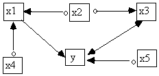
Fig. 5.32
From the POIPG it is possible to determine that relative to the set {x1, x2, x3, x4, x5, y}, x2, x3, and x4 are not direct causes of y, and x5 may or may not be a direct cause of y. We can also tell that x1 is a direct cause of y relative to {x1, x2, x3, x4, x5, y} because Build's output informs us that there is a directed path from x1 to y, and there are no directed paths from x1 to any of the other variables.