Input

This chapter describes TETRAD II input. Because it is intended chiefly as a reference to be consulted when needed, the chapter contains a description of any information that can be put into an input file or input interactively into the program. Many of the input sections are optional, or are required only by certain modules. Sections 4.1-4.5 should be read before proceeding further in the manual, but the user should feel free to skip the remaining sections until they are needed. In all cases, the chapters on individual modules indicate which sections of this chapter are relevant.

Overview

A TETRAD II input file is an unformatted, normal text file. It is organized into sections. For example, Fig. 4.1 is the input file "example.in," which has /Covariance and /Graph sections.

################# example.in ################

.in;..in;

/Covariance

2000

x1 x2 x3 x4 x5

1.5357

2.6924 6.7682

0.4044 1.2415 1.3159

0.6889 1.9295 0.5577 1.8057

0.8587 2.3956 0.6311 1.0173 2.1669

/graph

T x1

T x2

T x3

T x4

T x5

################# example.in #################

Fig. 4.1: The Input File "example.in"

For any particular TETRAD II process, most of the sections may be omitted, but which sections are necessary varies from module to module. The only restriction on the order in which the sections occur in the input file is that if there is a data section (i.e., /Covariance, /Raw, /Continousraw, /Independence, or /Cellcount), then it must be first, to be followed by a /Graph section, if there is one. After the optional /Graph section, the other sections can follow in any order. The possible sections are:

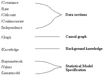
Fig. 4.2: Input File Sections

Sample data are entered in either the /Covariance, /Raw, /Cellcount, /Continuousraw or /Independence sections, whereas the causal structure is specified in the /Graph section. The /Knowledge section allows the user to enter background knowledge, for example, information about the time order of the measured variables. The /Bayesnetwork section allows the user to specify a fully parameterized Bayesian network, and the /Values section allows the user to specify the values of some of the variables in a Bayesian network when the goal is to use the network to compute conditional distributions. The /Linearmodel section specifies a linear recursive structural equation model for the Monte Carlo module.

Syntactic Conventions

Variable Names

The conventions for naming variables that appear in the input file are very simple.

• Any alpha-numeric character (i.e., any letter, upper-case or lower-case, and any digit) can be used in a variable name.

• Each variable name must be one to five characters long.

• Names for measured variable;s must begin with a lower case letter.

• Names for latent or unmeasured variables must begin with an upper case letter.^[1]

Examples of acceptable variables names are:

jobs

S1a2

The program interprets the last two names in the list as names of unmeasured variables. Examples of unacceptable variable names, with the accompanying reasons are:

1x begins with a digit instead of a letter

jobsalary more than five characters

SS_nu contains non-alpha-numeric character

In general, distinct variable names can be separated by any number of spaces or tabs.

Numbers

Numbers;

In any context other than names of variables, a legal number is an integer or a real number expressed as a decimal. It is not necessary to put a zero in front of a decimal point. TETRAD II does not read scientific notation, and commas should not be included in numbers. The maximum integer that can be read in the UNIX version is 65535. For the DOS version the largest integer that can be read is 32767. Any number of decimal places can occur after the decimal point, but the maximum number of decimal places that TETRAD II actually records is 15. In general, distinct numbers can be separated by any number of spaces or tabs.

Comments

An input file may contain a comment at the beginning of the file. Comments begin with a "{", end with a "}", and can include any number of lines of text. The program ignores any text that is anywhere on the same line as a closing bracket, "}" , even if the text occurs after the closing bracket.

File Names

The usual filename conventions apply to the DOS version of TETRAD II. That is, file names may have up to eight characters, followed by a ".", and then up to a three-character extension. If you give an extension with more than three characters, TETRAD II will truncate it to three.

You Enter: DOS Version of TETRAD II treats as:

file1 file1

file1.dat file1.dat

file2.data file2.dat

toobigname toobigna

Entering Input Files

TETRAD prompts for input file names interactively. You can tell it that you want to enter an input file name by typing the command: "input." It will then prompt for a filename, which you should type in and enter.

Session 4.1: Using the "Input" Command

******************************************************************

>input

Input File: example.in

Converting covariance matrix to correlation matrix.

The file example.in contains covariance data and a graph file. After reading the input file successfully, TETRAD II converts the covariances to correlations and then waits for a command.

*******************************************************************

Several input files containing different information can be entered in succession. If you issue some other command to TETRAD II and the input necessary for executing the command has not already been entered, the program will inform you what information it needs before it can proceed. For example, in session 4.2 the user wants to use the Monte Carlo generator, but has not yet entered a linear model or a Bayesian network (created with the Makemodel command).

Session 4.2

******************************************************************

>monte

MONTE requires either a linear model or a Bayesian network.

Fatal error: cannot proceed

*******************************************************************

If there is no input file corresponding to the name entered by the user, the program will re-prompt the user for another name. If the user wants to simply exit from the command without entering another name, simply press the "return" key (which we designate by "<CR>").

Session 4.3: Exiting from the "input" command

******************************************************************

>input

Input File: nofile

Could not open previous file.

Enter new input file name: <CR>

*******************************************************************

Data Sections

TETRAD II constructs two different kinds of models, linear structural equation models of continuous variables and Bayesian networks of discrete variables. Data for linear recursive structural equation models is always input in the form of a covariance or correlation matrix in a /Covariance section, or as raw continuous data in a /Continuousraw section. Data for discrete Bayesian networks is always entered in the form of raw data in a /Raw section, or cell counts in a /Cellcount section. If a model is neither linear nor discrete the user may tell TETRAD II what conditional independence relations hold in the distribution in an /Independence section. Entering any kind of data from an input file overwrites any other kind of data previously entered from a different file. A given input file cannot contain more than one of a /Covariance, /Raw, /Cellcount, /Continuousraw, or /Independence section. All of the variables that occur in any data section must begin with a lower case letter.

Entering covariance, discrete raw data, cellcount, independence, or continuous raw data into TETRAD II destroys several different kinds of information that may have been entered into the program previously. These include any initial graph, and several kinds of information relevant to the "Search" and "Build" commands (including temporal information (see section 4.6.4) and information about forbidden edges (see section 4.12.5). TETRAD II always issues a warning when prior information is erased. Of course, any erased information can be restored after the data is read in by issuing another "Input" command to read a file containing the information that was erased.

/Covariance

The user may enter either correlational data or covariance data in the /Covariance section.^[2] By a "number" we always mean a real number or integer. The correlations or covariances should be given in lower triangular form in the input file, as in Fig. 4.1.

The first line after the /Covariance section is an integer that represents the sample size. In the file "example.in" (Fig. 4.1) the sample size is 2,000. It occurs on a line by itself. After the sample size, there is a line that contains the names of the measured variables for which there is covariance data. The order of the variables on this line determines the order in which the covariances must be entered. For example, in "example.in" the covariance between x2 and x3 is 1.2415. The variable names are all separated by at least one space and can be placed over several lines, as long as no completely blank lines occur between two names.

The numbers following the list of variables begin on the next line, and represent the values of the covariances. The order of the numbers that follows the list of variable names obviously matters, but the spacing does not. It also does not matter what line a number occurs on (as long as there are no completely blank lines separating numbers.) TETRAD II will simply keep reading numbers until the lower triangle of the matrix has been completely filled. If fewer numbers than are needed to fill out the matrix have been entered into the covariance file, TETRAD II will issue an error message and refuse to process the data; if more numbers than are needed to fill out the matrix have been entered into the covariance file, then TETRAD II will issue a warning, but proceed normally. No latent variables may appear in the /Covariance section. Thus "T," which is a latent variable occurring in the /Graph section of "example.in" (because its name begins with an upper case letter), does not occur in the /Covariance section.

/Continuousraw

The /Continuousraw section is used to enter raw sample data for continuous variables. Each raw datum must be a real number. The raw data is used by the program to calculate a correlation matrix. On the UNIX version the sample size must be less than or equal to 50,000; on the DOS version the sample size must be less than or equal to 12,000. In both versions, the sample size must be greater than or equal to 4. Fig. 4.3 (example.raw) is an example.

/Continuousraw

x1 x2 x3

.2 .6 1.3

-10.2 .93 1.7

.5 .6 1.9

128.3 .2 -.45

43 .921 1.34

Fig. 4.3

After the section header, an integer representing the sample size occurs on a line by itself. After the sample size, there is a line that contains the names of the measured variables. The order of the variables on this line determines the order in which the data must be entered. The variable names are all separated by at least one space and may be spread over several lines, as long as no completely blank line separates any two variable names.

The data itself starts on a new line after the list of variable names. In Fig. 4.3, there are five lines following the list of variable names that contain the raw data for the values of the variables for each unit of the population. Thus in the first unit in the population (line 1 of data) x1 = .2, x2 = .6, and x3 = 1.3. There is currently no way to indicate that data is missing.

The program actually pays no attention to how the numbers are divided into lines. With these measured variables in the input, the program simply makes the 1^st, 4^th, and 7^th numbers entered the value of x1, the 2^nd, 5^th, and 8^thnumbers the values of x2, and so on.

/Raw

The /Raw section is used to enter data for discrete variables. Each raw datum must be an integer. In Unix the maximum number of different values for any discrete variable is 20. In the DOS version it is 10. On the UNIX version the sample size must be less than or equal to 50,000; on the DOS version the sample size must be less than or equal to 12,000. Fig. 4.4 (example.raw) is an example.

/Raw

x1 x2 x3

0 1 2

1 1 1

0 0 2

0 1 2

0 1 0

1 1 0

0 1 2

0 2 2

0 1 2

Fig. 4.4

The data itself starts on a new line after the list of variable names. In Fig. 4.4, there are 10 lines following the list of variable names that contain the raw data for the values of the variables for each unit of the population. Thus in the first unit in the population (line 1 of data) x1 = 0, x2 = 1, and x3 = 2. Each number must be between 0 and the maximum number of vertices (100 on the Unix version, 50 on the DOS version.) There is currently no way to indicate that data is missing.

Again the program actually pays no attention to how the numbers are divided into lines. With these measured variables in the input, the program simply makes the 1^st, 4^th, 7^th, etc. numbers entered the value of x1, the 2^nd, 5^th, 8^th, etc. numbers the values of x2, and so on. Thus instead of the input file in Fig. 4.4, TETRAD II will read equally well the input file shown in Fig. 4.5.

/Raw

x1 x2 x3

0 1 2 1 1 1 0 0 2

0 1 2 0 1 0

1 1 0

0 1 2

0 2 2

0 1 2

Fig. 4.5

/Cellcount

The /Cellcount section is another way to enter data for discrete variables. Rather than entering the value of each variable for each individual in the sample, /Cellcount records, for each possible combination of values of the measured variables, how many members of the sample have exactly that combination of values. A cell count is simply the number of units in the sample that have a given fixed set of values for the variables; that is, if there are three variables x1, x2, and x3 an example of a cell is x1 = 0, x2 = 0, x3 = 0. Consider the raw data in Fig. 4.6.

/Raw

x1 x2 x3

0 1 2

1 1 1

0 0 2

0 1 2

0 1 0

1 1 0

0 1 2

0 0 2

0 1 2

Fig. 4.6

There are 12 cells because x1 has two different values (0 and 1), x2 has two different values (0 and 1), and x3 has three different values (0, 1, and 2). The cell count for the cell x1 = 0, x2 = 0, x3 = 0 is zero, because there is no line with a 0 entry for x1, x2 and x3. The cell count for cell x1 = 0, x2 = 1, and x3 = 2 is 4 because the 1^st, 4^th, 8^th, and 10^th lines consist of a 0 entry for x1, a 1 entry for x2, and a 2 entry for x3. The cell count data list in Fig. 4.7 describes the raw data in Fig. 4.6.

x1 x2 x3 count

0 0 0 0

0 0 1 0

0 0 2 2

0 1 0 1

0 1 1 0

0 1 2 4

1 0 0 0

1 0 1 0

1 0 2 0

1 1 0 2

1 1 1 1

1 1 2 0

Fig. 4.7

However, Fig. 4.7 is not how the information would be entered in a TETRAD II input file. In Fig. 4.7, if the values for x1, x2, and x3 are concatenated together into a single number, the cell counts are given in numerical order; that is, the cell count for the first row 000 precedes the cell count for the second row R-what if out of order?001, and so on. The cell counts in Fig. 4.7 can be entered to TETRAD II as in Fig. 4.8.

/Cellcount

x1 x2 x3

2 2 3

0 0 2 1 0 4 0 0 0 2 1 0

Fig. 4.8

No sample size is specified; instead it is calculated from the cell counts. After the /Cellcount there is a new line that contains the names of the measured variables for which there is cell count data. The order of the variables on this line determines the order in which the cell counts must be entered. The variable names are all separated by at least one space and may be spread over several lines, as long as no completely blank line separates any two variable names. The next line specifies how many different values or levels the corresponding variable takes, for example, x1 and x2 take 2 values (0 or 1), and x3 takes 3 values (0, 1, or 2). The last line specifies the cell counts. On the UNIX version the sample size times sum of the cell counts must be less than 50,000; on the DOS version the sum of the cell-counts must be less than 12,000.

A concrete illustration may be useful. Coleman (1964).; described a study in which 3,398 schoolboys were interviewed twice. At each interview each subject was asked to judge whether or not he was a member of the "leading crowd" and whether his attitude toward the leading crowd was favorable or unfavorable. The data were reanalyzed by Fienberg (1977). Let a and b stand for the questions at the first interview and c and d stand for the corresponding questions at the second interview.

The data were given (Fig. 4.9) by Fienberg.; as follows:

Second Interview
Membership Attitude			+	+	-	-
			+	-	+	-
Membership Attitude
	+	+	458	140	110	49
First	+	-	171	182	56	87
Interview	-	+	184	75	531	281
	-	-	85	97	338	554

Fig. 4.9

The same data can be entered for TETRAD II as follows (Fig. 4.10):

i.Input files: coleman.dat;

################# coleman.dat ################

/cell

a b c d

2 2 2 2

458 140 110 49

171 182 56 87

184 75 531 281

85 97 338 554

################# coleman.dat #################

Fig. 4.10

The sequence of 2s in the second line tells the program each variable is binary. A carriage return must follow the final number.

/Independence

The Build algorithm uses decisions about conditional independence relations to build causal models. TETRAD II contains tests of conditional independence for two types of distributions: multinomial and multivariate normal. If the user has a sample distribution that is neither of these kinds, then TETRAD II has no way of testing for conditional independence. However, a user can perform her own tests of conditional independence, (e.g., R-check thisusing logistic regression) and this information can be entered directly into the program. An example is given in Fig. 4.11.

/independence

x1 x2 x3 x4

x1 x3

x1 x4 x2

x1 x3 x2

Fig. 4.11

The first line after /Independence is the list of variables in the sample distribution, in this case x1, x2, x3 and x4.^[3] Each line thereafter specifies an independence or conditional independence relation. The lines in this section correspond to the following independence facts:

Lines Independence Facts

x1 x3 x1 || x3

x1 x4 x2 x1 || x4 | {x2}

x1 x3 x2 x1 || x3 | {x2}

The /Graph Section

The /Graph section contains the specification of a causal graph. Fig. 4.12 shows an example of a /Graph section.

.in;

############# graph.in ###########

/graph

T x1

T x2

T x3

T x4

############# graph.in ###########

Fig. 4.12: The Input File "graph.in"

One specifies a directed graph to TETRAD after the /Graph section heading, one edge (e.g., "T x2") or one vertex (e.g., "x5") per line. Note that after the line "x5" there is a blank line, which is required.

If there is a /Graph section, it should follow any data section, and precede any other section. Each "/Graph" is followed by a list of lines containing information about the edges and vertices in the graph. The list is followed by a blank line that signals to the program the end of the list. The modules that require the user to input a graph are:

Estimate Tetrads Makemodel

Purify MIMBuild Search

Fig. 4.13: Modules that Require a /Graph Section

In addition, the Build module uses a /Graph section if the user chooses to enter it, but it is not required. Here we explain the syntax of the /Graph section. The use that each module makes of the /Graph section is explained in its own chapter.

TETRAD II represents causal structures by a directed acyclic graph, where there is a directed edge from x to y if and only if x is a direct cause of y. Each line in the graph consists of either a pair of vertices separated by at least one space or tab, or a single vertex. Upon reading a line that consists of a pair of vertices, TETRAD II adds the vertices read to the set of vertices in the graph, and also adds a directed edge from the first vertex to the second vertex in the graph. For example, in Fig. 4.12 the line "T x1" adds T and x1 to the set of vertices in the graph, and a directed edge from T to x1. The edge means that T is a direct cause of x1. Upon reading a single vertex on a line, TETRAD II simply adds the vertex to the set of vertices in the graph. It does not matter which edge is entered first, but of course it does matter, within each edge, which variable name is entered first. For example, the input file in Fig. 4.12 specifies the graph in Fig. 4.14.

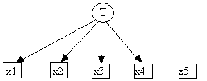
Fig. 4.14: The Causal Structure Specified by "graph.in"

Note that although the program always assumes that in linear structural equation models each variable is always also caused by a unique error variable, the error variables are not explicitly entered in the input file.

If data are entered as input, but no /Graph is explicitly input, the program constructs a default graph whose vertices are all of the variables appearing in the data, but without any edges. For example, given data about x1, x2, x3, x4, and x5, the program internally constructs the following default initial graph:

Fig. 4.15

Each time an input file is entered that contains a /Graph section, the previous graph will be erased entirely along with any other knowledge that has been entered, with the possible exception of previously entered data. The /Graph section will not wipe out previously entered data unless the graph contains a measured variable that does not occur in the data. If some previous knowledge that has been erased because of entry of a /Graph section, the knowledge can be read back in after the /Graph section has been read.

Graphs with Linear Coefficients

In a linear structural equation model associated with a graph, each variable is a linear function of its direct causes (parents) in the graph and a unique error variable. Consider the following /Graph section:

/graph

T x1

T x2

T x3

T x4

x2 x1

Fig. 4.16: A /Graph Section Without Linear Coefficients

The structural equations corresponding to this graph are:

x₁ = a_T,x1T + a_x2,x1x2 + e_x1

x₂ = a_T,x2T + e_x2

x₃ = a_T,x3T + e_x3

x₄ = a_T,x4T + e_x4

where the a_ij terms are unspecified but constant real-valued coefficients. Particular values can be assigned to these coefficients in the /Graph section by adding a number after an edge. For example:

/graph

T x1 .2

T x2

T x3 1.3

T x4 -2.1

x2 x1 3.22

Fig. 4.17: A /Graph Section With Linear Coefficients

This /Graph section now corresponds to the following set of structural equations, where the a_T,x2 coefficient is left unspecified:

x1 = .2 T + 3.22 x2 + e_x1

x2 = a_T,x2T + e_x2

x3 = 1.3 T + e_x3

x4 = -2.1 T + e_x4

In general, if a line in a graph section consists of "v1 v2 num" then "num" is the coefficient of "v1" in the structural equation for "v2."

The /Knowledge Section

The /Knowledge section is used to set parameters that guide the search conducted by various modules. Because there are a large number of such parameters and the meaning of the parameters depends on understanding what each module does, we explain the meaning of these parameters in the chapters that describe the modules. This section should be skipped until the relevant chapters on the modules have been read. Here we will simply describe what parameters can be specified in the /Knowledge section and the syntax required to do so.

Real-Valued Parameters

The following parameters take numerical values, with the specified default values, and must be within the given range:

Parameter Default Range Used By

Settime -1.0 (Unbounded) -1..60000.0 Build, Search

Significance 0.05 0..1.0 Build, Search,

MIMbuild, Purify

Weight 0.1 0..1000.0 Search, MIMbuild,

Purify

Width 0.95 0..1.0 Search

Fig. 4.18

To set the value of one of these parameters simply place the desired real value for the parameter after the name of the parameter, separated by at least one space. Fig. 4.19 shows how to set the values of these parameters from a file(example.knowledge).

/Knowledge

Settime 20

Significance .8

wei .3

wid .20

Fig. 4.19

If there is an error in the specification of the value of the parameter in the file the program will inform you of what type of error occurred, and leave the value of the parameter unchanged. Each of these parameters can also be set interactively, instead of from a file. Simply type the name of the parameter that you desire to set; the program then prints out the current value of the parameter, and prompts you to enter a new value. If you type a <CR> the value is not changed. If you type an illegal value, the program will prompt you to re-enter a correct value. Session 4.4 shows interactions for the "Weight" parameter.

Session 4.4: Setting Real-Valued Parameters

*******************************************************

>weight

Weight [ 0.1000 ]: .2

>we

Weight [ 0.2000 ]: -17

Warning:

Number less than lower bound of 0.0000

Weight [ 0.2000 ]: 1

*******************************************************

Integer Valued Parameters

The following parameter takes an integer value, with the specified default values, and must be within the given range:

Parameter Default Range Used By

Depth -1 (Unbounded) -1..100 Search

Decimals 4 0..8 Statwriter, Monte, Makemod

To set the value of the depth parameter or the decimals parameter simply place the desired integer value for the parameter next to the name of the parameter, separated by any number of spaces or tabs. The decimals parameter determines how many numbers are printed after a decimal point in Tetrad II output. If an integer valued parameter is given a real value instead of an integer value, it will be rounded off to the nearest integer. Fig. 4.20 illustrates how to set these values.

/Knowledge

Depth 2

Decimals 4

Fig. 4.20

Boolean Valued Parameters

The following parameters take on either the values "Yes" or "No":

Parameter Default Used By

Acyclic Yes Search

Common Yes Search

Ll Yes Search

Lm Yes Search

Ml Yes Search

Mm Yes Search

Singleconnection Yes Search

Fig. 4.21: Boolean Valued Parameters

To set the value of one of these parameters simply place the desired value (yes or no) for the parameter next to the name of the parameter, separated by any number of spaces or tabs. Either upper-case or lower-case letters can be used. (The program actually uses only the first letter to determine whether the value is Yes or No; any string beginning with a 'y' or a 'Y' is interpreted as yes, and anything else is interpreted as no.) For example, see Fig. 4.22. Again, each of these parameters can also be set interactively, instead of from a file.

/Knowledge

Acyclic NO

Common N

Ll n

Lm yes

Ml Y

Mm N

Singleconnection No

Fig. 4.22: Setting Boolean Parameters

Addtemporal and Removetemporal

The Addtemporal and Removetemporal commands are used to enter information about the time order in which variables are known to occur. The information is used by the Search and Build commands. Suppose x67 and y67 were measured in 1967, x72 and y72 were measured in 1972, x84 was measured in 1984, and the temporal relationship of z1 to the other variables is not known. (These variables must previously have been mentioned in a /Graph, /Raw, /Covariance, /Cellcount, or /Independence section.) No model that suggests an edge from a later variable to an earlier variable should be allowed. These models can be eliminated from consideration by the Build or Search command in the following way using the Addtemporal command:

/Knowledge

addtemporal

1 x67 y67

3 x84

2 x72 y72

Fig. 4.23

Following the Addtemporal command is a list of lines, specifying the temporal information. After the last line in the list, the user must leave a blank line, indicating that the addtemporal command has ended. In this example, the line "2 x72 y72" is followed by a blank line. Each line consists of a number followed by a tab or a space, and a list of variables separated by at least one space or tab. The first number on each line is an index used to determine which set of variables precedes which other set of variables; a set of variables indexed by a lower number precedes a set of variables indexed by a higher number. The temporal information is stored in an indexed array of sets of variables. The first set of variables in the array is x67 and y67; the second set of variables is x72 and y72, and the third set of variables is x84. (Note that x72 and y72 is in the second set of variables because it is indexed by the number 2, even though it occurs after the line describing the third set of variables.) After the line "2 x72 y72" a blank line must occur, indicating that the "Addtemporal" command is ended.

No information about the temporal relationships of variables appearing on the same line is stored. Each variable can be indexed by at most one number. It would be incorrect to place x67 in the set indexed by 1 and the set indexed by 2. It is not necessary to place all of the variables in some indexed set of variables. Note that z1, whose temporal relationship to the other variables is not known, is not placed in any of the sets. To remove a variable from a given indexed set of variables, simply call the "removetemporal" command (Fig. 4.24). For example, the /Knowledge section in Fig. 4.24 removes the variable x72 from the set of variables indexed by 2:

/Knowledge

removetemporal

2 x72

Fig. 4.24

It is also possible to use the Addtemporal and Removetemporal commands interactively. After either of these commands is invoked, the program prints the current indexed sets of variables and then gives an example of a syntactically correct line of input. The user is then repeatedly prompted to enter a number and a list of variables until a blank line is entered to indicate that no more information is to be entered. Then the program prints out the current indexed sets of variables (including the changes that have just been entered.) For example:

Session 4.6: Using addtemporal and removetemporal interactively

*********************************************************

>addtemp

In this case there is no temporal information yet, so the program prints an example of an input line and then prompts for temporal information.

Example of input:

1 x67 y67 x72

Temporal tier: 1 x67 y67

Temporal tier: 2 y72 x72

Temporal tier: 3 x84

Temporal tier: <CR>

Temporal Tier: 1

x67 y67

Temporal Tier: 2

y72 x72

Temporal Tier: 3

x84

>removetemp

Temporal Tier: 1

x67 y67

Temporal Tier: 2

y72 x72

Temporal Tier: 3

x84

In this case there is a temporal order stored in the program, so TETRAD II prints out the temporal tiers, gives an example of an input line, and then prompts for temporal information.

Example of input:

1 x1 x2 x3

Temporal tier: 2 y72

Temporal tier: <CR>

Temporal Tier: 1

x67 y67

Temporal Tier: 2

x72

Temporal Tier: 3

x84

**********************************************************

Forbidding Edges and Common Causes

Temporal restictions are implemented in the program as forbidden edges. That is, if x1 and x2 are both listed in temporal tiers, and x1's tier is prior to x2's, then the program will not consider models in which x2 is a direct cause of x1. Edges can be forbidden directly, however. Two commands, Forbiddirect and Forbidcommon, are used to specify edges or common causes (correlated errors) that the user wants the Search or Build commands to not include in any of the output models. The commands Allowdirect and Allowcommon undo the restraints imposed by Forbiddirect and Forbidcommon, however they cannot undo edges forbidden by temporal tiers. (The variables mentioned in these commands must previously have been mentioned in a /Graph, /Raw, /Covariance, /Continuousraw, /Cellcount, or /Independence section.) The commands are included in the /Knowledge section, followed by the edges they should operate on. For example, suppose the initial graph is as specified in Fig. 4.25

/Graph

T x1

T x2

T x3

T x4

T x5

Fig. 4.25

If background knowledge indicates that x1 cannot cause x2, x2 cannot cause x3, and that there is no common cause (correlated errors) of x3 and x4, then one way to enter these restrictions is as follows:

/Knowledge

Forbiddirect

x1 x2

x2 x3

Forbidcommon

x3 x4

Fig. 4.26

The first line of the command states what sort of causal connection is being forbidden, a direct edge in the first case, and a common cause in the second case. There must be a blank space after the last edge in each list. Each edge in the list is specified as the cause followed by at least one space followed by the effect. The Allowdirect command acts in an analogous fashion, but undoes the effect of a Forbiddirect command.

These commands can also be used interactively. Suppose that the /Graph section is that of Fig. 4.25, stored in the file example2.in.

Session 4.6: Using forbiddirect and forbidcommon interactively

*********************************************************

>forbiddirect

Example of input:

x1 x2

Edge: x1 x2

Edge: x2 x3

Edge: <CR>

>forbidcommon

Example of input:

x1 x2

Edge: x3 x4

Edge: <CR>

*************************************************************

The /Bayesnetwork Section

This section is used to store a discrete Bayesian network.^[4] A Bayesian network is a directed acyclic graph that represents a factorization of a probability distribution. In a discrete Bayesian network G over a set of variables V, the joint distribution over V is the product of the conditional distribution of each child on its parents in G, that is:

(where the direct causes of x in a causal graph are the parents of x).

Suppose for example that a Bayesian network is represented by the graph in Fig. 4.27.

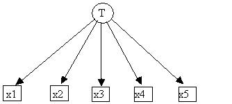
Fig. 4.27

In this case

P(x1,x2,x3,x4,x5,T) = P(T) ´ P(x1|T) ´ P(x2|T) ´ P(x3|T) ´ P(x4|T) ´ P(x5|T)

Hence the joint distribution can be determined from P(T), P(x1|T), P(x2|T), P(x3|T), P(x4|T) and P(x5|T). This information is entered into the program from the file example2.bn:

################ example2.bn ###############

/BAYESNETWORK.bn;.bn;

Number of Values of

Variable Categories Categories

T 2 0 1

x1 2 0 1

x2 2 0 1

x3 2 0 1

x4 2 0 1

x5 2 0 1

The Probability Distribution

----------------------------

T Parents:

p(T=0)= 0.5823 p(T=1)= 0.4176

----------------------------

x1 Parents: T

when T=0

p(x1=0)= 0.1786 p(x1=1)= 0.8213

when T=1

p(x1=0)= 0.7461 p(x1=1)= 0.2539

----------------------------

x2 Parents: T

when T=0

p(x2=0)= 0.7269 p(x2=1)= 0.2730

when T=1

p(x2=0)= 0.6705 p(x2=1)= 0.3295

----------------------------

x3 Parents: T

when T=0

p(x3=0)= 0.4375 p(x3=1)= 0.5625

when T=1

p(x3=0)= 0.0313 p(x3=1)= 0.9687

----------------------------

x4 Parents: T

when T=0

p(x4=0)= 0.6147 p(x4=1)= 0.3853

when T=1

p(x4=0)= 0.9528 p(x4=1)= 0.0471

----------------------------

x5 Parents: T

when T=0

p(x5=0)= 0.7373 p(x5=1)= 0.2627

when T=1

p(x5=0)= 0.3257 p(x5=1)= 0.6743

################ example2.bn ###############

Fig. 4.28

According to this distribution, P(T = 0) = .5283; P(x1 = 0|T = 0) = .1786, and so on. Because the structure of this input section is complex, we recommend that you do not create it from scratch. Instead, Makemodel helps you write a Bayesian network in the proper format. See chapter 12.

The /Linearmodel Section

/graph

T x1 0.5916

T x2 0.6497

T x3 0.4310

T x4 0.4243

T x5 0.5075

.lm;.lm

/linearmodel

Variable Dist. Type Parameters

x1 Normal 0.0000 1.0000

x2 Uniform 0.0000 2.0000

x3 Normal 0.0000 1.0000

x4 Normal 2.0000 3.000

x5 Normal 0.0000 1.0000

T Normal 0.0000 1.0000

Fig. 4.29

The /Graph section specifies the causal graph and the linear coefficient corresponding to each edge in the graph. In the TETRAD II representation of a linear structural equation model, every variable has an independent error term, and the /Linearmodel section specifies the distribution over these errors. TETRAD II allows two distributional families, normal and uniform. The normal takes mean and variance as parameters, and the uniform takes an upper and lower bound. For more detail, see chapters 12 and 13.

^[1]The character "Z" is treated as a special character by the STATwriter module. See chapter 14.

^[2]We mean "correlation or covariance" whenever we say "covariance."

^[3]The list of variables may cover several lines. TETRAD II interprets the list of variables to be ended when it comes across a variable that has already occurred in the list, in this example, when it finds the second occurrence of x1, which occurs on the second line after the "/independence."

^[4]See chapter 2 for an explanation of Bayesian networks.