Theoretical Foundations
Introduction
The theory upon which TETRAD II rests is presented in more detail in Causation, Prediction and Search (Spirtes, Glymour, and Scheines 1993). In this chapter we attempt only to provide enough detail so that the program can be used with good scientific sense.
TETRAD II deals with statistical models explicitly meant to represent causal processes. We take as primitive the notion of direct causation among variables, which is a relative concept: one variable is a direct cause of another only relative to a system of variables. For example, in a system of two variables, match strikings and match lightings, match strikings are a direct cause of match lightings. If we include match tip temperature, however, then match strikings are only an indirect cause of match lightings. We represent the set of direct causal relationships among a system of variables C with a directed graph interpreted causally, i.e., a causal graph.
Statistical causal inference is the task of inferring features of the causal processes that generated data from statistical properties of the sample and background knowledge. It is sometimes the case that very little can be learned about causal structure from measured data. If we have measured only two variables x and y, for example, and find that they are associated, then under the assumptions we endorse we know only that x is a cause of y, y of x, or some other variable is a cause of both, or x and y are related in multiple ways. This example underlies the oft heard adage: "correlation does not imply causation," but it does not imply that it is impossible to learn anything about causal structure from patterns of statistical association. In some cases you can learn quite a lot.
Statistical Causal Models
A directed graph consists of a set of vertices V, and a set of directed edges between the vertices. We will sometimes refer to directed acyclic graphs (that is directed graphs that contain no directed paths leading from a variable x back to x) as DAGs. A directed graph G is a causal graph for C if there is a directed edge from x to y in G if and only if x is a direct cause of y relative to C. Fig. 2.1 is an example of a causal graph.

Fig. 2.1
TETRAD II handles two classes of statistical causal models: 1) Linear Structural Equation Models (SEMs), which are used widely in economics, biometrics, psychometrics, market research, political science, sociology, and elsewhere, and 2) Discrete Bayesian networks, which are used in artificial intelligence, medical expert systems, and increasingly in the social sciences.
We will begin by discussing these models, and present axiomatically the connection between causal structure and probability distributions that these models share. We will then include a section on the vanishing tetrad difference, a constraint that is particularly useful in connecting the causal structure of SEMs that involve latent (unmeasured) variables with probability distributions. We then discuss the difference between predicting the values of variables in two kinds of systems, those that have been manipulated and those that have not. We will explain why knowledge of causal structure is crucial to the former. We conclude with a discussion of the limitations of the TETRAD II methods.
Linear Structural Equation Models[1]
A linear structural equation model (SEM) is a system of linear equations and some statistical constraints. The equations in a SEM are considered "structural" if their form corresponds to the causal processes among the variables being modeled. Conventionally, each variable y is given on the left hand side of a structural equation and is set equal to a linear combination of its direct causes and an "error" term ey. In some treatments, a constant is included in the structural equations, but in linear models we can eliminate the constant term without loss of generality by recording the means and expressing each variable as the difference from its mean. In this treatment we follow that strategy, but never deal with the means explicitly. The path diagram, or causal graph, for a structural equation model gives the direct causes for each effect (all the variables that have an arrow into the effect).

Fig. 2.2
For example, the structural equations associated with the causal graph in Fig. 2.2 are:
Structural Equations
x1 = e1
x2 = e2
x3 = a*x1
+ b*x2 + e3
x4 = c*x3 +
e4
where a, b, and c are real valued constants not equal to 0, and each unit in the population is governed by the same structural equations. It is assumed that the error terms are independently and identically distributed, that the first and second moments of all error terms exist and are finite, and that the second moment (variance) of an error term is never zero. Unless specified otherwise, ei and ej are assumed to be independent for all i, j, and if so we do not include them in our diagrams. If ei and ej are dependent, then they are included in the diagram and connected with an undirected line, for example, e3 and e4 in Fig. 2.3.
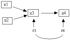
Fig. 2.3: e3 and e4 dependent
Such an undirected line represents an unspecified causal connection between the error terms. The set of covariance matrices that can be generated from different parameterizations of the model in Fig. 2.3 is the same as the set that can be generated from different parameterizations of the model in Fig. 2.4, in which the correlated errors are replaced with a latent common cause of x3 and x4 but the error terms e3' and e4' are uncorrelated. Because all of TETRAD II's procedures work on directed graphs, the program requires the latent common cause representation of a correlated error in its input files.
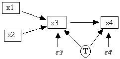
Fig. 2.4
Informally, a directed path is a chain of arrows x ® y ® z ® w linked head to tail.[2] A structural equation model is recursive if there are no "cycles" in its path diagram, that is, there are no directed paths that go from a variable back to itself. RSEM is an abbreviation for "linear recursive structural equation model."
The joint distribution among the non error variables V in an RSEM is determined by the triple <G, D(e), f>, where G is the causal graph over V, D(e) is the joint distribution among the error terms e, and f the linear coefficients that correspond to each arrow in the path diagram. All of the TETRAD II procedures that analyze RSEMs take as input either a covariance (or correlation) matrix, or raw data, and assume a multivariate normal distribution. If the covariance matrix is not input directly, then raw data is converted to a correlation matrix before it is analyzed. Under these assumptions (and in some cases much weaker ones) several statistical packages[3] will provide a maximum likelihood estimate of D(e) and f for models that are identifiable.
In order to construct graphs representing causal structures, TETRAD II uses judgements about independence constraints in the population in the Build module, and judgements about vanishing tetrad differences in the population in the Purify, MIMbuild, and Search modules.
Under the assumption of multivariate normality, a test of zero correlation or zero partial correlation is also a test of independence or conditional independence respectively. That is, rxy.C = 0 Û x || y | C, where the expression x || y | C denotes "x is independent of y conditional on the set C", and rxy.C is the partial correlation of x and y controlling for C.
Discrete Bayesian Networks
In the sort of Bayesian networks TETRAD II can handle, the variables must all range over a discrete set of values. In a Bayesian network there are no error terms, so instead of expressing each effect as a function of its direct causes and an error, we express the probability distribution of each effect as a function its direct causes. The joint distribution over the variables V in a discrete Bayesian network can be factored according to the causal structure in the following way:
![]()
(According to our convention for causal graphs, y is a direct cause of x if and only if there is an edge y ® x in the causal graph, i.e. the direct causes of x are the parents of x in the causal graph.) For example, the hypothetical causal structure in Fig. 2.5 might be interpreted as a Bayes network in which each of the variables is binary valued, for example, true or false. In that case the joint distribution over s, y, and c factors:
P(s,y,c) = P(s) P(y|s) P(c|s)
and we can parameterize the network by giving the distribution of each effect for each array of possible values its causes might take on.
smoking and lung cancer;
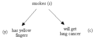
Fig. 2.5: Causal Graph
Suppose that if someone smokes we assign them s = 1, and 0 otherwise, if they will get lung cancer we assign them c = 1, and 0 otherwise, and if they have yellow fingers we assign them y = 1, and 0 otherwise. One parameterization of this Bayesian network is:
P(s = 1) = .34
P(s = 0) = .66
P(y = 1| s = 1) = .7 P(y = 0| s = 1) = .3
P(y = 1| s = 0) = .1 P(y = 0| s = 0) = .9
P(c = 1| s = 1) = .16 P(c = 0| s = 1) = .84
P(c = 1| s = 0) = .03 P(c = 0| s = 0) = .97
Calculating the products from this factorized distribution gives the joint distribution in conventional form:
P(y = 1, s = 1, c = 1) = .03808 P(y = 0, s = 1, c = 1) = .01632
P(y = 1, s = 1, c = 0) = .19992 P(y = 0, s = 1, c = 0) = .08568
P(y = 1, s = 0, c = 1) = .00198 P(y = 0, s = 0, c = 1) = .01782
P(y = 1, s = 0, c = 0) = .06402 P(y = 0, s = 0, c = 0) = .57618
Latent Variables and Causal Sufficiency
So far we have discussed models over a set of random variables V, and represented the direct causal relations among V with directed edges in a causal graph over V. We include a directed edge from y to z Î V just in case y is a direct cause of z relative to V.
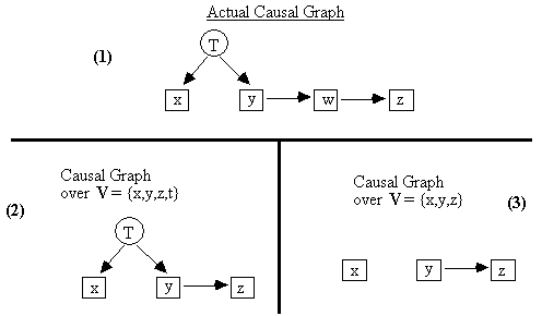
Fig. 2.6
Suppose that in the true causal graph (part 1 of Fig. 2.6), T is a common cause[4] of x and y, and that this is the only form of causal connection between x and y, but T is not included in V = {x,y,z}. Then according to our conventions, the causal graph over {x,y,z} will include no edge at all between x and y (part 3 of Fig. 2.6).
If a set of variables V includes all the common causes of pairs of variables in V, then we say V is causally sufficient. In Fig. 2.6 above, for example, the set {x,T,y,z) is causally sufficient, while the set {x,y,z} is not. The latter leaves out T, which is a common cause of x and y. The exact set of causally sufficient sets among {x,T,y,w,z} for the actual causal graph in Fig. 2.6 is:
{T}, {x}, {y}, {w}, {z}
{T,x}, {T,y}, {T,w}, {T,z}, {y,w}, {y,z}, {w,z}
{T,x,y}, {T,x,w}, {T,x,z}, {T,y,w}, {T,y,z}, {T,w,z}, {y,w,z}
{T,w,y,z}, {x,T,y,w}, {x,T,y,z}, {x,T,w,z},
{x,T,y,w,z}
Fig. 2.7 : Causally Sufficient Sets for the Actual Graph in Fig. 2.6
Causal sufficiency matters for representation and for inference. Henceforth, whenever we draw a causal graph we will assume that the set of variables in the graph, both measured and unmeasured, are causally sufficient unless we explicitly include correlated errors. This assumption will enable us to articulate a general connection between causal graphs and the probability distributions they can produce, and we discuss this connection in the next section. TETRAD II's procedures and the interpretation of their output is affected by whether or not the set of measured variables is assumed to be causally sufficient. In the Build module, for example, you are required to choose between assuming or not assuming causal sufficiency for the measured variables. Naturally, the causal conclusions one can make are in general stronger if it is assumed that the measured variables are causally sufficient than if it is not.
Causal Structure and Probabilistic Independence
The Markov Condition
The connection between causally sufficient causal structures and the set of independence and conditional independence relations in the probability distributions they can generate is the same for RSEMs and Bayesian networks and is given by the Markov condition. (We assume that in an RSEM with a causally sufficient set of variables, that the error terms are jointly independent.) A variable x is a descendant of y in a directed graph G if and only if there is a directed path from y to x, or y = x. Suppose that we have a causally sufficient set of variables V, a probability distribution P over V, and a causal graph with vertices V. Then P satisfies the Markov condition for G if and only if in P, each variable v is independent of every set of variables that does not contain v or its descendants, conditional on v's direct causes (i.e. v's parents in the causal graph).[5]
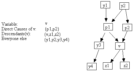
Fig. 2.8
For example, if the causal graph in Fig. 2.8 and a distribution P satisfy the Markov condition, then {v} || {y1, y2, y3, y4} | {p1, p2} in P.
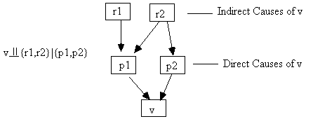
Fig. 2.9: Direct Causes Screen Off Indirect Causes
Two intuitive consequences of the Markov condition are that (a) an effect is independent of its indirect causes conditional on its direct causes (Fig. 2.9), and (b) that variables are independent conditional on their common causes (Fig. 2.10).

Fig. 2.10: The Principle of the Common Cause
The Markov condition is assumed, even if not always explicitly, in many branches of statistics. It is assumed in many analyses of latent variable models (e.g., Bartholomew, 1987) and special cases of the condition are fundamental to the theory of experimental design (Spirtes, Glymour, & Scheines, 1993).
Faithfulness
As we have seen, if we assume the Markov condition, then we can deduce from the causal graph of an RSEM or a Bayesian network some conditional independence relations in the population. These conditional independence relations hold regardless of what the particular parameter values in the RSEM or Bayesian network are. In this case we say that the causal graph entails those conditional independence relations. Both types of models induce independence constraints on the population due to the Markov condition, and RSEMs induce an extra set of constraints (discussed in section 2.6 below) because they are linear. It does not follow, however, that every constraint found to hold in a population governed by some causal structure is entailed by that causal structure. For example, if a probability distribution satisfies the Markov condition for the causal graph in Fig. 2.11, there are some parameterizations of the causal graph in which the tax rate is not independent of tax revenue. However, in a parameterization in which the two causal paths from tax rate to tax revenue (one negative and the other positive) exactly balance, tax revenue is independent of tax rate.
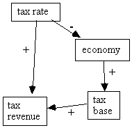
Fig. 2.11
It requires unusual circumstances for the two paths to cancel exactly, however. Under the class of measures absolutely continuous with Lebesgue measure, the set of RSEM parameterizations that balance the two causal paths from tax rate to tax revenue exactly has measure 0. In general, the set of parameterizations of an RSEM that produce an independence relation or vanishing tetrad difference not implied by every parameterization of its causal structure is Lebesgue measure 0 (Spirtes, Glymour, & Scheines, 1993).
If a distribution P over a causally sufficient set of variables is generated by a model with causal graph G, and P satisfies the Markov condition for G, and all the conditional independence constraints that hold in P hold in any Bayesian network or RSEM parameterization of G (i.e. they entailed by G) then we say the pair <G,P> are faithful, and that P satisfies the Faithfulness condition for G. Unless we state otherwise, in tasks of causal inference we assume that a distribution over a causally sufficient set of variables generated by a causal structure with causal graph G, is faithful to G.
Markov Equivalent Models
Many distinct causal graphs entail the same independence and conditional independence constraints, so if our only data were these independence and conditional independence constraints we could not distinguish among such causal structures. If two models entail the same set of independence constraints, then we say they are Markov equivalent. Under the assumption of causal sufficiency, the Build procedure outputs a set of Markov equivalent models and represents them with a pattern.[6]
The graph-theoretic characterization of Markov equivalence is simple, and forms one sort of precise bound on the limits of causal inference from independence constraints. Only two concepts need be defined, adjacency and unshielded-collider.
x and y are adjacent in a causal graph G iff:
1) x is a direct cause of y (i.e., x is a parent of y in the causal graph) or
2) y is a direct cause of x (i.e., y is a parent of x in the causal graph).
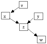
Fig. 2.12
If x and y both directly cause z, then we say z is a collider on any undirected path containing x ® z ¬ y. A variable is a collider on a path, however, and can be a collider on one path and a non collider on another. In Fig. 2.12, for example, z is a collider on any path containing x ® z ¬ y but a non-collider on any path containing x ® z ® w.

Fig. 2.13
If x and y are not adjacent, then we say z is an unshielded collider on any undirected path containing x ® z ¬ y (Fig. 2.13). If a path contains x ® z ¬ y, but x and y are adjacent, then we say z is a shielded collider on any such path. Indistinguishability is now easy to characterize:[7]
Markov Equivalence Theorem: Two acyclic causal graphs over the same variables entail the same conditional independence relations (by applying the Markov condition) if and only if (a) they have the same adjacencies, and (b) the same unshielded colliders.
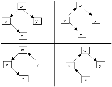
Fig. 2.14: Markov Equivalent Causal Graphs
For example, the graphs in Fig. 2.14 are Markov equivalent, but the causal graphs in Fig. 2.15 all entail distinct sets of independence constraints.
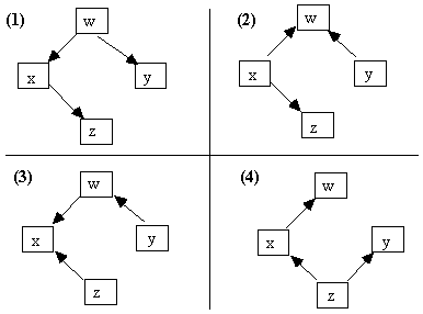
Fig. 2.15: Distinguishable Causal Graphs
Detecting Latent Variables
By assuming that a distribution satisfies the Markov and Faithfulness conditions for the graph of a causal structure, it is sometimes possible to detect latent variables. Certain patterns of conditional independence relations among a set of variables V cannot be generated by any DAG with just the variables in V. For example suppose that V = {x1, x2, x3, x4} and the only conditional independence relations that hold in the distribution P over V are x1 || {x3,x4} and x4 || {x1,x2}. No DAG containing only the variables in V entails these two and only these two independence relations. Under the assumption that P satisfies the Markov and Faithfulness conditions for the graph of the causal structure that generated it, we can infer that the causal graph that generated the distribution contains some variable T that is not in V, and moreover that T is a common cause of x2 and x3. Fig. 2.16 shows a DAG with a latent common cause T that entails x1 || {x3,x4} and x4 || {x1,x2}, and entails no other independence or conditional independence relations among just the variables in V.
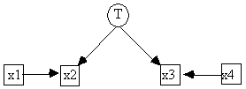
Fig. 2.16
Vanishing Tetrad Differences
Because of linearity, the causal structure of an RSEM induces constraints on the population that a Bayesian network with the same causal structure might not. One such constraint is the vanishing tetrad difference.
A tetrad difference among four variables is the determinant of a 2x2 sub-matrix of the covariance or correlation matrix involving just those four variables. A tetrad difference that vanishes is a tetrad equation or a vanishing tetrad difference. For example, there are three tetrad equations among x1, x2, x3, and x4, any two of which are independent:
rx1,x2 * rx3,x4 = rx1,x3 * rx2,x4 = rx1,x4 * rx2,x3
Recall that an RSEM can be parameterized by <G, D(e), f>, where G is the causal graph, D(e) is a distribution over the exogenous variables, and f is a vector of the coefficients in the linear functions. An RSEM's causal graph G entails a constraint t, for example, a tetrad equation or vanishing partial correlation, when t holds for all values of <f, D(e)>. (Remember that we are assuming that for a causally sufficient set of variables the error terms are jointly independent). Although we use statistical tests of vanishing tetrad constraints that assume joint normality, the tetrad constraints themselves are entailed under the assumption of linearity, even without the assumption of normality. For example, consider the RSEM whose causal graph is shown in Fig. 2.17.
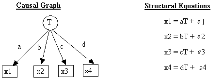
Fig. 2.17
Assuming, without loss of generality, that the mean of each variable is 0, we can derive a tetrad constraint from this model among x1 - x4 with simple covariance algebra, where gx,y is the covariance between x and y, and Var(x) is the variance of x.
gx1,x2 = E(x1x2) - E(x1)E(x2)
= E(x1x2)
= E[(aT + e1)(bT + e2)]
= E[abT2 + aTe2 + bTe1 + e1e2]
= abE(T2) + aE(Te2) + bE(Te1) + E(e1e2)
= abE(T2)
= ab Var(T)
gx3,x4 = cd Var(T)
gx2,x3 = bc Var(T)
gx1,x4 = ad Var(T)
gx1,x2 ´ gx3,x4 = abcd Var2(T) = adbc Var2(T) = gx1,x4 ´ gx2,x3
So for all values of a,b,c,d and Var(T):
gx1,x2 ´ gx3,x4 - gx1,x4 ´ gx2,x3 = 0
The Tetrad
Representation Theorem (Spirtes, 1989) is a graph theoretic characterization of
when an RSEM's causal graph implies a tetrad constraint, and this
characterization underlies the Purify, MIMbuild, and Search modules. Vanishing
tetrad differences are most useful in models that have unmeasured or latent
variables. When latent common causes are operative the set of independence
relations true of the measured marginal is often not very informative. For
example, if the measured variables V
= {x1, x2, x3, x4}, then none of the models in Fig. 2.18 imply any independence
or conditional independence relations among V.

Fig. 2.18
If, however, we assume that the model in which x1, x2, x3, and x4 are embedded is an RSEM, then we can use tetrad constraints to distinguish between these models. The tetrad constraints entailed by each of the four models in Fig. 2.18 are:
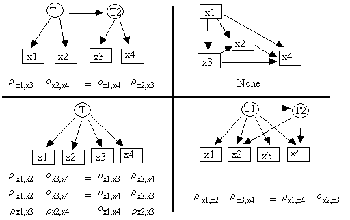
Fig. 2.19
There is a corollary of the Tetrad Representation Theorem that provides a simple test for the existence of latent common causes, which is implemented as part of the Build module:
Tetrad Representation Corollary: If ri,jrk,l - ri,lrj,k = 0 for all parameterizations of an RSEM's causal graph G, then either ri,j or rk,l = 0, and ri,l or rjk = 0, or there is a (possibly empty) set Q such that ri,j.Q = rk,l.Q = ri,l.Q = rj,k.Q = 0, and neither {i,k} nor {j,l} is a subset of Q.
Suppose we measure only V
= {x1, x2, x3, x4}, and we want to know if there is a latent common cause of
the variables in V. If a tetrad
equation t holds non trivially[8]
among the variables in V, then if
the distribution is faithful there must be a Q Í V such that each correlation involved in t vanishes when partialled on Q.
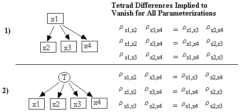
Fig. 2.20
Fig. 2.20 shows two causal graphs that cannot be distinguished by the tetrad equations they imply, but Fig. 2.21 shows how they can be distinguished by the existence of such a set Q Í V. In model 1 in these figures, Q = {x1}, so we do not need to postulate a latent variable. In model 2, however, there is no such Q containing only measured variables; hence we postulate the existence of a latent variable.
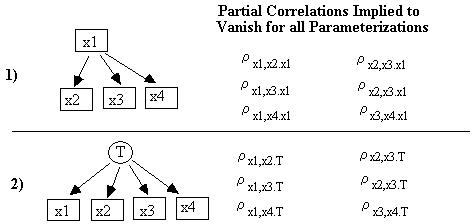
Fig. 2.21
When applied to covariance data, the Build module gives information about foursomes for which this corollary applies, that is, foursomes that are all effects of a latent common cause (see chap. 5).
Causation, Prediction, and Manipulation
Causal knowledge is critical in predicting the results of a manipulation (Robins, 1986 & 1989), for example, the change in economic growth when the Federal Reserve reduces interest rates. If the population we wish to study is one which we will not manipulate, and our goals are only to classify or forecast, then information about the statistical associations, without regard to the causal mechanisms or processes that may have produced those associations, is sufficient. In this section we work through a simple example to make this difference concrete. A more detailed discussion is given in Causation, Prediction, and Search, (Spirtes, Glymour, & Scheines, 1993, chap. 7).
Consider again the simple example we used in section 2.2.2. Smoking cigarettes causes both nicotine stains and lung cancer.

Fig. 2.22
Suppose we interpret this causal structure as a Bayesian network in which each of the variables is binary valued, for example, true or false. In that case we can parameterize the network by giving the distribution of each effect for each array of possible values its causes might take on. For example:
P(s = 1) = .34
P(s = 0) = .66
P(y = 1 | s = 1) = .7 P(y = 0| s = 1) = .3
P(y = 1 | s = 0) = .1 P(y = 0| s = 0) = .9
P(c = 1| s = 1) = .16 P(c = 0| s = 1) = .84
P(c = 1| s = 0) = .03 P(c = 0| s = 0) = .97
Fig. 2.23
This Bayesian network about smoking can be used to calculate the chances that someone chosen at random has lung cancer:
P(c = 1) = P(c = 1 | s = 1) * P(s = 1) + P(c = 1 | s = 0) * P(s = 0)
= .16 * .34 + .03 * .66 = .0742
It can also be used to calculate conditional probabilities, for example, the chances that someone with hands free of nicotine stains has lung cancer:
P(c = 1 | y = 0) = [P(y = 0, s = 1, c = 1) + P(y = 0, s = 0, c = 1)] / P(y = 0)
= [.016 + .018] / .696 = .04905
These calculations can be performed as long as the joint distribution is known, and several different causal structures could be parameterized to produce exactly this joint distribution. One important use of knowing a causal structure along with a joint distribution is in predicting the effect of manipulations. To manipulate a variable (yellowed fingers) is to force it to take on a certain value. When we force a variable to take on a particular value, we are essentially breaking the causal links into it. So, for example, if we force a heavy smoker with nicotine stained hands to wash his hands until they are stainless, we have changed the causal structure that would be found "naturally." For example, Fig. 2.24 shows the changes in causal structure from Fig. 2.22 that would result from forcing everyone to wash their hands until stainless.

Fig. 2.24: Manipulating Nicotine Stains
The changes in the probability distribution that result from this sort of manipulation can be made precise. The manipulated distribution PM, that is, the distribution that corresponds to the manipulated causal structure, preserves the conditional probabilities among variables connected by unbroken links from the pre-manipulated distribution, but forces the manipulated value on the manipulated variable. In this case the manipulation does nothing to s, nor to the link between s and c, so the probabilities involving s and c alone are unchanged:
PM(s = 1) = .34
PM(s = 0) = .66
PM(y = 0) = 0 PM(y = 1) = 1.0
PM(c = 1 | s = 1) = .16 PM(c = 0 | s = 1) = .84
PM(c = 1 | s = 0) = .03 PM(c = 0 | s = 0) = .97
This distribution and not the original one is used to predict the effect of the manipulation M. For example, PM(c = 1) is the probability that someone has lung cancer given that he or she was forced to wash their hands until they were stainless. And because
PM(c = 1) = PM(c =1 | s = 1) * PM(s = 1) + PM(c = 1| s = 0) * PM(s = 0)
= .16 * .34 + .03 * .66
= .0742,
you can see that PM(c = 1) ≠ P(c = 1 | y = 0). That is, the probability of getting lung cancer after everyone is forced to obtain stainless hands is not the same as the conditional probability of getting lung cancer given that your hands are stainless.
Suppose that the true causal structure were not as we believe it to be, but were instead as we show in Fig. 2.25. Suppose further that this structure was parameterized so that the joint distribution was identical to the one in Fig. 2.22.[9] The same manipulation would not remove any links in the graph, and in this case the probability of lung cancer in the manipulated population would be the same as the conditional probability of lung cancer on stainless hands in the unmanipulated distribution, that is, PM(c = 1) = P(c = 1 | y = 0).

Fig. 2.25
The joint distribution over the variables V in a discrete Bayesian network can be factored according to the causal structure in the following way:
![]()
For discrete variables, given a correct graphical description of a premanipulated causal structure and corresponding probabilities, the effects of an ideal intervention that forces a new distribution PM(x) on x can be calculated directly by substituting PM(x) in for P(x|Direct Causes of x). Given a correct graphical description of a premanipulated causal structure and the corresponding equations in an RSEM, if an ideal intervention forces the value x upon a variable x, the new distribution can be calculated by replacing the equation for x in terms of its direct causes by the equation x = x.
Of course, not every manipulation to change the value of a variable only breaks causal links into the manipulated variable. It is possible that some interventions to change the value of a variable also introduce new causal links or otherwise alter the structure. Interventions of this kind lie outside of the scope of the theory just described.
Limitations
In general, the correctness of the output of the model building modules in TETRAD II depends upon six factors:
1. The correctness of the background knowledge input to the algorithm.
2. Whether the Markov Condition holds.
3. Whether the Faithfulness Condition holds.
4. Whether the distributional assumptions made by the statistical tests hold.
5. The power of the statistical tests against alternatives.
6. The significance level used in the statistical tests.
We do not have a formal mechanism for combining these factors into a score for the reliability of the output, but we will make some informal remarks about them.
1. Each of the algorithms in TETRAD II allows the user to put constraints upon the search conducted by the program. If the assumptions are incorrect, there is obviously no guarantee that the output of the program is correct. We suggest that if you are not sure whether the background information that you input to the program is correct, that you run the program with several different alternative inputs. For example, when using the Search module, a user might start from several different plausible initial models.
2. The Markov Condition holds in a wide variety of circumstances, but it does not hold universally. In particular, it does not hold in any of the following kinds of cases.
A. "Population" effects: Sometimes the value of a variable for one unit of the population causes the value of a variable for a different unit in the population. For example, the probability that one person gets an infectious disease depends upon whether or not others around him have the disease.
B. Mixtures of populations in which causal connections are in opposite directions: During a given period of time, some people may be exposed to a chemical because of their employment status, and some people may change their employment status because of their exposure to the chemical. It is possible that some people drink too much because they are depressed, and other people are depressed because they drink too much. A mixture of units in which the causal connections go in opposite directions does not in general satisfy the Markov Condition.
C. Cyclic processes reaching equilibrium: This occurs when we measure the value of all the random variables at one time, but the process by which the values of the random variables were generated alternated between a variable A at time t causing the value of variable B at time t+1, and the value of variable B at time t + 1 causing the value of a variable A at t + 2, and so on. This may happen for example in a wage-price spiral that comes to rest at some equilibrium. Such an equilibrium distribution does not in general satisfy the Markov Condition.
D. Nonrandom samples: It is possible that if a sample is not representative of the population, then statistical constraints in the sample will be different from statistical constraints in the population. For example, a survey questionnaire may only be returned by people who are not typical of the population. If the people who return the survey all share the same value of some variable z, and this variable is caused by other variables x and y being measured, this can lead to statistical dependencies between x and y in the sample, even though x and y are independent in the population. In many cases, it will be obvious from the sampling scheme used that this might have occurred.
3. The Faithfulness Condition can be violated when there are deterministic relationships among the variables. For this reason, one should never include in a set of variables submitted to TETRAD II any variable that is definable in terms of other variables in the set. For example, if the G.N.P for the U.S. is defined to be the sum of the G.N.P's for each state, one should not include both the G.N.P's for each state and the national G.N.P. Of course there may be deterministic relationships among variables even when none of the variables are definable in terms of the other variables. You should not apply TETRAD II to sets of variables in which in the linear case there are correlations very close to 1, or in the discrete case where there are conditional probabilities very close to 1.
Unfortunately, there are also cases where the Faithfulness Condition may be violated because of deterministic relationships, but it is not possible to determine from the measured data alone that it has been violated. Consider the following hypothetical causal graph, where a, b and sexual anatomy are measured phenotypic traits but the Y chromosome variable is unmeasured.
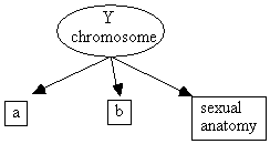
Fig. 2.26
The Markov Condition entails that a and b are independent given the value of Y chromosome, but it does not entail that a and b are independent given sexual anatomy. However, if the probability of having a Y chromosome given male sexual anatomy is equal to one, and the probability of not having a Y chromosome given female sexual anatomy is equal to one, then a and b are also independent given sexual anatomy. That this is a violation of faithfulness is not detectable from the marginal distribution over a, b, and sexual anatomy. Note that the violation of faithfulness is not due to being able to perfectly predict sexual anatomy from the Y chromosome, but from being able to perfectly predict the value of the latent Y chromosome from sexual anatomy.
4. TETRAD II gets information about conditional independence relations in the population either from lists of conditional independence relations given by the user or by performing statistical tests. If variables are continuous, the tests are only correct if the variables are jointly normal. There are standard tests for joint normality that should be performed upon the variables. If the variables cannot be transformed into a joint normal distribution, it is still possible to run TETRAD II, and it may provide useful suggestions; however, the output is obviously less reliable than if the distributional assumptions are satisfied. In the study on causes of publishing productivity, we applied TETRAD II to a set of variables that violated the joint normality condition (because gender is binary), but the program nonetheless produced plausible suggestions very similar to those models proposed by Rogers and Maranto. At this time, we do not have any measure of how sensitive TETRAD II is to deviations from normality and linearity although in practice, statistical tests based on the assumption of normality are still often useful for nonnormal distributions.
It may appear then that it would be best always to discretize variables. There are two reasons for not doing so. First, the statistical tests that we employ for discrete variables are not very powerful against alternatives, and need large sample sizes to be useful. The second reason is that even when the output of the program is correct for discretized variables, it may not be very informative. For example if z is a continuous variable, and x and y are independent conditional on z, they might not be independent conditional on z', a discretized version of z. A statistical test may then correctly determine that x and y are dependent on z', but the valuable information that x and y are independent conditional on z will be missed.
5. In general, very small effects are not detectible except at very large sample sizes. The power of the algorithm against alternatives is an unknown and extremely complex function of the power of the statistical tests that we employ. For that reason, the best answer that we can give about the reliability of the algorithm is based upon simulation studies. We have provided the results of a variety of simulation tests in the individual chapters describing the modules. The simulation studies should be interpreted as an upper bound on the reliability of the program, because in general the distributional assumptions made by the program are exactly satisfied in the simulations, and if a causal connection exists between variables in a study, we have limited how weak that causal connection can be.
Under ideal circumstances, and in the limit as the sample size approaches infinity, the output of the TETRAD II algorithms (with the exception of the "Search" module, which is heuristic) is reliable (if the significance level is systematically lowered as the sample size increases). However, in practice, the circumstances under which it is actually applied will not be ideal, nor will the sample sizes be infinite. We suggest that you interpret the output of TETRAD II as plausible suggestions for further investigation. We recommend that wherever possible the models output by TETRAD II be estimated and subjected to a variety of measures of how well the data fits the suggested model. In the case of linear structural equation models this can be done by such programs as CALIS, EQS, or LISREL. (The "Statwriter" module of TETRAD II will help you translate the TETRAD II output into input for these programs.) The user should keep in mind however, that even when a model suggested by TETRAD II fits the data very well, it is possible that there are other models that will also fit the data well and are equally compatible with background knowledge, particularly when the sample size is small. R- think about thisAlso, at large sample sizes, even slight deviations from normality or linearity can lead to the rejection of an otherwise correct model. Finally, there is a selection bias when models are tested on the same data that they are constructed from, so p(c2) is best interpreted as a measure of fit.