Regress
15.1 Introduction
We distinguish two kinds of predictions that can be made. First, one may try to predict the value of some variable, given the values of other variables. This is typically what is done in diagnostic problems. Given symptoms, one tries to determine what disease is present. Alternatively, one may try to predict the value of some variables, given the values of other variables, after the causal structure has been interfered with in some prescribed way. This is typically what is attempted when various policies are compared. Linear regression is a useful technique for answering the first kind of question; the regressee is the variable whose value is being predicted, and the regressors are the variables used to make the prediction.
One problem associated with linear regression is how to choose the set of regressors. There may be several reasons for choosing a small set of regressors. First, it may be costly to measure the values of a large set of regressors. Second, when a regression equation is estimated on one sample, but used to predict the value of a variable on a different sample, a smaller set of regressors can sometimes lead to a smaller mean squared error on the new sample than does a larger set of regressors. (This is in contrast to the case where a regression equation is estimated on one sample and used to predict the value of a variable on the same sample; in that case, increasing the number of regressors cannot lead to a larger mean squared error.)
The Regress Module can be used to automatically select a set of regressors, and then estimate the regression coefficient. It does not perform any action that could not be produced by an ordinary regression package, and we have provided it mainly so that users may perform regressions without exiting TETRAD II.
15.2 Using the Regress Module
Given either raw continuous data or a covariance matrix as input, the Regress module first selects a set of regressors, and then estimates the regression coefficients. Consider the following example. The input can be either a covariance matrix, as in Figure 15.1, or raw data, as in Figure 15.2.
############### man1.dat
##############
Covariance Matrix
x1 x2
x3 y x5
x6 x7 x8
1.3774
0.8128 1.4531
1.0235 0.6281 1.7797
2.4842 2.4959 2.5278 6.9852
-0.0031 -0.0025 -0.0120
-0.0030 0.9784
2.8692 2.8569 2.8980 8.0385 0.8287 10.9764
0.5964 0.3585 0.4455 1.0916 0.0124 1.2721 0.9768
2.7941 2.8113 2.8112 7.8674 0.8375 10.7494 1.2314 11.5255
############### man1.dat
##############
Fig. 15.1: Covariance Matrix
############### man.dat
##############
/continuousraw
5000
x1
x2 x3 y
x5 x6 x7
x8
-0.9380
-0.7871 1.1391 1.2430 -1.5807 1.0637 0.6399 1.5263
0.4573 -0.7920 0.3312 0.3593 0.3567 -0.3029
0.6204 0.0890
-0.1869
-0.1715 -0.2845 0.0111 -1.2424 -3.2048 -0.1505-2.2447
0.0931 -0.3288 -0.0543 -1.4286 0.2749 -1.9362
-0.0455 -0.8420
.
.
############### man.dat
##############
Fig. 15.2: Raw Data
Session 15-1 illustrates how to use the Regress module.
Session 15-1.
*****************************************
>in
Input File: man.dat
Converting covariance
matrix to correlation matrix.
To start Regress, simply type regress at the prompt.
>regress
Output file: man.out
Name of regressee: y
>exit
*****************************************
We show the relevant portions of the file man.out in Fig. 15.3:
########## man.out ##############
Regression Coefficients
Intercept 0.0035
x1 0.2957
x2 0.4655
x3 0.2863
x5 -0.4120
x6 0.4894
TSS = 34927.7954
RegrSS = 32778.6744
RSS = 2148.8056
R-squared = 0.9385
##########
man.out ##############
Fig. 15.3: Regress’s Output (cooper.out)
The output can be interpreted in the following way. The regression equation is:
y = 0.0035 + 0.2957 x1 + 0.4655 x2 + 0.2863 x3 - 0.4120 x5 + 0.4894 x6
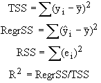
If yi is the value of y on the ith unit in the sample, ![]() is the mean of y,
is the mean of y, ![]() is the value of yi predicted from the regression equation,
and ei is the difference
between yi and
is the value of yi predicted from the regression equation,
and ei is the difference
between yi and ![]() , then the following quantities can be defined:
, then the following quantities can be defined:

The quantities defined
above can only be calculated when TETRAD II is given a sample (rather than just
a covariance matrix), so they are only output when the data is given in a /Continuousraw
section.
15.3 Selection of Regressors
Given a multivariate normal distribution, TETRAD II selects a set of regressors for a variable y by first calling the Build module to form either a pattern or a POIPG, and then applies an algorithm to the output to select the regressors. In the large sample limit, we conjecture that the regressors chosen are precisely those variables that have non-zero coefficients when y is regressed upon the set of all other variables.
One obvious alternative to the method used by TETRAD II to select regressors is to simply regress y on all other variables, and remove each variable which passes a statistical test that its coefficient is equal to zero. In the large sample limit, these two methods will select the same regressors; however, in small samples, the sets of regressors selected by the two different methods may differ. One theoretical advantage of using the Regress module rather than the alternative method described above is that the Regress module selects regressors using low order conditional independence tests, while the alternative method implicitly tests higher order conditional independence relations. In small samples, the former are more reliable than the latter. However, we do not currently know whether this theoretical advantage translates into a practical advantage.