STATwriter: A Statistical Package Input File Writer
14.1 Introduction
TETRAD II helps to specify linear recursive structural equation models, but it does not estimate the parameters of these models, calculate standard errors, or perform statistical tests of their fit. There are several commercial packages already available that perform these functions, for example, LISREL, EQS, and CALIS (a SAS PROC).[1] To save time and trouble, TETRAD II has a module that will convert a TETRAD II input file into an input file for any of these packages. STATwriter requires two input sections:
1. A /Graph section.
2. A /Covariance or /Continuousraw section.
For example, the /graph section in the file stat1.g represents the causal structure of the model in Fig. 14.1.
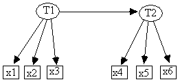
Fig. 14.1
Makemodel can then be used to create a fully parameterized linear model from this structure, and the Monte Carlo Generator to create a pseudo-random sample from this model, which we store in the file stat1.dat (Fig. 14.2):
################# stat1.dat #################
{
The
Generating Model
Linear
Structural Equation Model
Distribution
over exogenous variables
Error Distributional
term for
Family
Parameters
--------
--------------
----------
x1 Normal Mean:
0.0000 Variance: 1.0000
x2 Normal Mean:
0.0000 Variance: 1.0000
x3
Normal Mean: 0.0000
Variance: 1.0000
x4
Normal Mean: 0.0000
Variance: 1.0000
x5
Normal Mean: 0.0000
Variance: 1.0000
x6
Normal Mean: 0.0000
Variance: 1.0000
T1
Normal Mean: 0.0000
Variance: 1.0000
T2
Normal Mean: 0.0000
Variance: 1.0000
Structural
Equations
--------------------
T1
= e7
T2
= 1.213T1 + e8
x1
= 0.874T1 + e1
x2
= 0.655T1 + e2
x3
= 1.222T1 + e3
x4
= 0.842T2 + e4
x5
= 0.749T2 + e5
x6
= 0.815T2 + e6
}
/Covariance
2000
x1 x2
x3 x4 x5 x6
1.0000
0.3323
1.0000
0.5180
0.3975 1.0000
0.4085
0.3477 0.4840 1.0000
0.3885
0.3191 0.4509 0.6122 1.0000
0.4084
0.3106 0.4668 0.6307 0.6202 1.0000
/graph
T1
T2
T1
x1
T1
x2
T1
x3
T2
x4
T2
x5
T2
x6
#################
stat1.dat #################
Fig. 14.2: The TETRAD II input file stat1.dat
This file contains a comment in which the generating model is written, a /Covariance section, and finally a copy of /Graph section from stat1.g. Converting this TETRAD II input file into an input file for EQS, CALIS and LISREL is straightforward. We show the interaction in session 14.1.
Session 14.1: Making EQS,
LISREL, and CALIS input files
*************************************************
>input
Input File: stat1.dat
>statwriter
STATwriter prompts for which packages we want input files. Here we choose all three.
1 = EQS Input File
2 = LISREL Input File
3 = SAS\CALIS Input File
List the types of input files you want below.
Separate each number by a space, and
use no delimiters. List = 1 2 3
Name
of EQS input file that
TETRAD
II will create: [eqs.in]stat1.eqs
If
you wish, enter a comment for the input file
*Generated by tetrad
Name
of LISREL input file that
TETRAD
II will create: [lisrel.in]stat1.lis
If
you wish, enter a comment for the input file
*Generated by tetrad
Name of SAS/CALIS input file that
TETRAD II will create: [calis.in]stat1.cal
If you wish, enter a comment for the input file
*Generated
by tetrad
>exit
*************************************************
TETRAD II creates the EQS input file in Fig. 14.3, the LISREL input file in Fig. 14.4, and the CALIS input file in Fig. 14.5.
############ stat1.eqs
############
/TITLE
Generated
by tetrad
/SPECIFICATIONS
CAS
= 2000;
VAR
= 6;
/LABELS
V1
= x1; V2 = x2; V3 = x3; V4 = x4; V5 = x5; V6 = x6;
F1
= T1; F2 = T2;
/EQUATIONS
V1
= 1.0
F1 + E1;
V2
= 0.0000*F1 + E2;
V3
= 0.0000*F1 + E3;
V4
= 1.0
F2 + E4;
V5
= 0.0000*F2 + E5;
V6
= 0.0000*F2 + E6;
F1
= D1;
F2
= 0.0000*F1 + D2;
/VARIANCES
E1 = 0.5*;
E2
= 0.5*;
E3
= 0.5*;
E4
= 0.5*;
E5
= 0.5*;
E6
= 0.5*;
D1
= 0.5*;
D2
= 0.5*;
/MATRIX
1.0000
0.3323
1.0000
0.5180
0.3975 1.0000
0.4085
0.3477 0.4840 1.0000
0.3885
0.3191 0.4509 0.6122 1.0000
0.4084
0.3106 0.4668 0.6307 0.6202 1.0000
/END
############ stat1.eqs
############
Fig. 14.3: The EQS Input File stat1.eqs
############ stat1.lis
############
Generated
by tetrad
Observed
Variables x1 x2 x3 x4 x5 x6
Covariance
Matrix
1.0000
0.3323
1.0000
0.5180
0.3975 1.0000
0.4085
0.3477 0.4840 1.0000
0.3885
0.3191 0.4509 0.6122
1.0000
0.4084
0.3106 0.4668 0.6307
0.6202 1.0000
Sample
Size 2000
Latent
Variables T1 T2
Relationships
x1
= 1*T1
x2
= T1
x3
= T1
x4
= 1*T2
x5
= T2
x6
= T2
T2
= T1
End
of Problem
############
stat1.lis ############
Fig. 14.4: The LISREL Input File stat1.lis
############ stat1.cal
############
DATA TETDATA(TYPE=COV);
TITLE "Generated by tetrad";
_TYPE_ = 'COV'; INPUT _NAME_ $V1-V6;
LABEL V1 = 'x1' V2 = 'x2' V3 = 'x3' V4 = 'x4' V5 =
'x5' V6 = 'x6'
F1 = 'T1' F2 = 'T2' ;
CARDS;
V1
1.0000 . . . .
V2
0.3323 1.0000 .
. . .
V3
0.5180 0.3975 1.0000
. . .
V4
0.4085 0.3477 0.4840
1.0000 .
V5
0.3885 0.3191 0.4509
0.6122 1.0000 .
V6
0.4084 0.3106 0.4668
0.6307 0.6202 1.0000
;
PROC
CALIS DATA=TETDATA COV EDF=1999;
TITLE2
"Generated by tetrad";
LINEQS
V1
= F1 + E1,
V2
= X1 ( 0.0000 ) F1 + E2,
V3
= X2 ( 0.0000 ) F1 + E3,
V4
= F2 + E4,
V5
= X3 ( 0.0000 ) F2 + E5,
V6
= X4 ( 0.0000 ) F2 + E6,
F1
= D1,
F2
= X5 ( 0.0000 ) F1 + D2;
STD
E1 = THE1 (0.5),
E2 = THE2 (0.5),
E3 = THE3 (0.5),
E4 = THE4 (0.5),
E5 = THE5 (0.5),
E6 = THE6 (0.5),
D1 = THE7 (0.5),
D2 = THE8 (0.5);
RUN;
############ stat1.cal ############
Fig. 14.5: The SAS/CALIS Input File stat1.cal
14.2 Specifying Starting Values
One can give these statistical packages starting values for the parameters to be estimated. Unfortunately, the iterative estimation procedures are often sensitive to these starting values. In many cases the iterations will not converge, not because of the structure of the model specified, but because of the starting values of the parameters to be estimated. LISREL 8 automatically chooses starting values-consult your user manual for more information. We describe the way in which starting values are assigned by TETRAD II when creating an input file for anyone of the statistical estimation packages and how one can change these starting values, but we use an input file for the EQS package to explain the concepts.
In an EQS input file, starting values of parameters to be estimated are followed by a "*." For example, in the last line of the /EQUATIONS section in the EQS input file in Fig. 14.3, the coefficient (shown below in boldface) describing the linear dependence of F2 (EQS's name for T2) on F1 (T1) is started at 0, and is free to be estimated.
F2 = 0.000*F1 + D2;
The TETRAD II default for all starting values for the linear coefficients is 0.0, and 0.5 for all the variances to be estimated. If you wish to change any of these you can simply edit the regular text input file TETRAD II creates before submitting the file to EQS, LISREL, or CALIS. Alternatively, you may specify starting values for the linear coefficients in /graph section of the TETRAD II input file that is used to create the input file for your statistical estimation package. To specify a starting value for the linear coefficient associated with any edge in the /graph section of a TETRAD II input file simply add the starting value to the same line on which the edge is specified. For example, the /graph section in stat2.g (Fig. 14.6) fixes two coefficients.
############ stat2.g ############
/graph
T1
T2 .75
T1
x1
T1
x2 1.2
T1
x3
T2
x4
T2
x5
T2
x6
############ stat2.g ############
Fig. 14.6
This will change the /EQUATIONS section of the EQS input file produced (stat2.eqs), as we show in Fig. 14.7. We highlight the affected coefficients in boldface, although they are not in boldface in the actual file.
############ stat2.eqs
############
/EQUATIONS
V1 =
1.0 F1 + E1;
V2 = 1.2000*F1 + E2;
V3 =
0.0000*F1 + E3;
V4 =
1.0 F2 + E4;
V5 =
0.0000*F2 + E5;
V6 =
0.0000*F2 + E6;
F1 = D1;
F2 = 0.7500*F1 + D2;
############ stat2.eqs
############
Fig. 14.7
14.3 Fixing Scales
The numerical scale for a latent variable is arbitrary. In specifying an input file for a statistical estimation package, one can fix a scale for each latent variable involved in the model in one of two ways:
1. Fix the variance of the latent and the sign of one edge from the latent to one of its effects.
2. Fix one coefficient associating the latent to one of its effects.
STATwriter takes the second strategy. For each latent variable T in the /graph section input, the STATwriter fixes the coefficient expressing the dependence on T of exactly one of T's effects. For example, in the input files already given, the equations involving x1 and x4 fix the factor loadings at 1. In Fig. 14.8 we give the first four lines in the relevant sections from each of the input files already given.
EQS
/EQUATIONS
V1 =
1.0 F1 + E1;
V2 =
0.0000*F1 + E2;
V3 =
0.0000*F1 + E3;
V4 = 1.0 F2 + E4
LISREL
Relationships
x1 = 1*T1
x2 = T1
x3 = T1
x4 = 1*T2
CALIS
LINEQS
V1 = F1 + E1,
V2 = X1 (
0.0000 ) F1 + E2,
V3 = X2 (
0.0000 ) F1 + E3,
V4 = F2 + E4,
Fig. 14.8: Fixing Factor Scales
One fixes a parameter in an EQS input file by omitting the * after the starting value for the coefficient. Accordingly, the coefficient associated with the dependence of the measured variable V1 (x1) on F1 (T1) is fixed at 1.0 to choose F1's scale, and the other two coefficients are free to be changed from their starting value of 0.5. LISREL and CALIS have parallel conventions.
14.4 Correlating Error Terms
In structural equation models each variable is a function of its direct causes and an error term. One can specify that the error terms associated with a pair of variables are correlated. This is represented graphically by an undirected curve, as we show between the error terms for x3 and x4 in model A of Fig. 14.9.
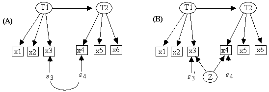
Fig. 14.9
The set of covariance matrices one can generate from a linear model in which the error terms associated with x3 and x4 are correlated is exactly the same as the set that can be generated from a model in which a new latent variable is introduced as a common cause of x3 and x4, and the error terms for x3 and x4 are uncorrelated (Fig. 14.9, model B). Because all of TETRAD II's procedures work on directed graphs, it employs the latent common cause representation of a correlated error. Since it is more convenient to specify models for the statistical packages we discuss here by correlating error terms, we provide a way for STATwriter to read a graph file with a latent common cause but write an input file in which a pair of error terms are correlated. If, in the /Graph section of a TETRAD input file, there is a latent variable (a) whose name begins with Z, and (b) that is a common cause of at least two non "Z" variables, then in the input file for the statistical estimation package, the STATwriter will ignore the latent, but correlate the error terms associated with every pair of its effects. For example, the /Graph section in stat3.g (Fig. 14.10) represents the TETRAD graph in Fig. 14.9.B.
####################
stat3.g ####################
/graph
T1 x1
T1 x2
T1 x3
T2 x4
T2 x5
T2 x6
T1 T2
Z x3
Z x4
####################
stat3.g ####################
Fig. 14.10: /Graph of Model B in Fig. 14.9
Given a TETRAD II input file with this /graph section, and a covariance matrix or raw continuous data, the STATwriter produces the EQS input file stat3.eqs, which we show in Fig. 14.11 (only the relevant sections are shown). Notice that the variable Z is not included in the file, but the appropriate error terms, e3 and e4, are correlated in the /Covariance section.
############ stat3.eqs ############
/EQUATIONS
V1
= 1.0
F1 + E1;
V2
= 0.0000*F1 + E2;
V3
= 0.0000*F1 + E3;
V4
= 1.0
F2 + E4;
V5
= 0.0000*F2 + E5;
V6
= 0.0000*F2 + E6;
F1
= D1;
F2
= 0.0000*F1 + D2;
/VARIANCES
E1
= 0.5*;
E2
= 0.5*;
E3
= 0.5*;
E4
= 0.5*;
E5
= 0.5*;
E6
= 0.5*;
D1
= 0.5*;
D2
= 0.5*;
/COVARIANCES
E3,E4 = 0.5*;
############ stat3.eqs
############
Fig. 14.11
14.5 Uncorrelated Exogenous Variables in LISREL
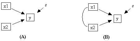
Fig. 14.12
The only difference between the two models in Fig. 14.12 is that in model (A) the exogenous variables x1 and x2 are constrained to be uncorrelated while in model (B) they are allowed to covary. That is, in model (A) Cov(x1,x2) = 0 while in model (B): Cov(x1,x2) ≠ 0. Imposing such a constraint can change the maximum likelihood estimate of the parameters representing the dependence of y on the x variables, so it ought to be possible to impose it. STATwriter creates LISREL files in the SIMPLIS format, however, and constraining exogenous variables to be uncorrelated in SIMPLIS is not straightforward. For example, if the two Relationships section in Fig. 14.13 were given to LISREL 8, it would treat both as if it were estimating the model in Fig. 14.12 (B), that is, it would allow x1 and x2 to covary.
(A) (B)
Relationships Relationships
y = x1 x2 y = x1 x2
Set the covariance of x1 and x2 to 0
Fig. 14.13
In general, one cannot specify that exogenous measured variables are uncorrelated in SIMPLIS. It is possible to specify that exogenous latent variables are uncorrelated, however, and therefore STATwriter's strategy is to create a surrogate latent variable for any measured exogenous variable that is specified to be uncorrelated with some other exogenous variable. For example, the following input file (lis1.in) will estimate the parameters of the model in Fig. 14.12 (A) under the constraint that Cov(x1,x2) = 0.
################## lis1.in #################
Observed Variables x1 y x2
Latent Variables Ksi1 Ksi2
Relationships
y = Ksi1 Ksi2
x1 = 1*Ksi1
x2 = 1*Ksi2
Set the Error Variance of x1 to 0
Set the Error Variance of x2 to 0
Set the Covariances of
Ksi1 and Ksi2 to 0
End of Problem
################## lis1.in
#################
Fig. 14.14
For each measured variable xi that we need to constrain to be uncorrelated with another variable, STATwriter creates a surrogate latent variable Li that is identical to xi. It then constrains the surrogate Li to be uncorrelated with other latent variables and other surrogate latents. To create such an Li, SIMPLIS requires two lines in the Relationships section:
xi = 1*Li
Set the Error Variance of xi to 0
The first line fixes the coefficient between xi and Li
at 1, and the second makes the relationship deterministic. In the example in Fig. 14.14, x1 and x2 are
constrained to be uncorrelated by the line: Set
the Covariances of Ksi1 and Ksi2 to 0
You need not impose the constraint that exogenous variables are uncorrelated. After selecting the LISREL option from the STATwriter menu, you are prompted for whether you want to impose this constraint or not:
Exogenous variables
uncorrelated? [y]
The default is yes, so if you want to STATwriter to write a SIMPLIS input file in which all exogenous variables will be free to covary in the model LISREL actually estimates, simply type "n."
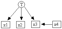
Fig. 14.15
Another example that involves a specified latent (T) as well as a surrogate latent (Ksi1) shows how things can get a little complicated. STATWriter will create the file lis2.in (Fig. 14.16) for the model shown in Fig. 14.15. Only x4 and T are exogenous, and so in order to impose the constraint that they are uncorrelated, only x4 needs a surrogate latent.
############## lis2.in ####################
Observed Variables x4 x3 x1 x2
Latent Variables T Ksi1
Relationships
x3 = Ksi1 1*T
x1 = T
x2 = T
x4 = 1*Ksi1
Set the Error Variance of x4 to 0
Set the Covariances of
Ksi1 and T to 0
##############
lis2.in ####################
Fig. 14.16
Joreskog and Sorbom (1993a) describes restrictions that the SIMPLIS language places on the kinds of models that can be estimated. In our limited experience, using LISREL with SIMPLIS input works well with pure multiple indicator models, and path models with correlated errors. However, there are some other kinds of models which LISREL accepts as syntactically correct, but on which it fails to produce informative output.