The Monte Carlo Generator
13.1 What It Does
The TETRAD II Monte Carlo Generator produces pseudo-random samples from populations described by recursive linear structural equation models or Bayesian networks. The program will produce raw sample data, a sample covariance or correlation matrix, or (in the linear case) a population covariance or correlation matrix.

Fig. 13.1
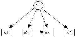
For example, having specified the causal structure shown in Fig. 13.1 in the /Graph section of the input file monte1.g, and having used Makemodel to randomly parameterize a linear model with this causal structure (monte1.lm, Fig. 13.2), the Monte Carlo Generator can be used to create a pseudo-random sample and store it in monte1.dat (Fig. 13.3), which itself is readable as a TETRAD II input file.
############ monte1.lm
###########
/graph
x2 x3 0.4270
T x1 0.3792
T x2
0.5403
T x3
0.5696
T x4
0.7639
/linearmodel
Variable
Dist. Type Parameters
x1 Normal 0.0000 1.0000
x2 Uniform 0.0000 2.0000
x3 Uniform 2.0000 6.0000
x4 Normal 0.0000 2.0000
T Normal 0.0000 1.0000
############ monte1.lm
###########
Fig. 13.2
############ monte1.dat ###########
{
The Generating Model
Linear
Structural Equation Model
Distribution
over exogenous variables
Error
Distributional
term
for Family Parameters
-------- -------------- ----------
x2
Uniform Lower: 0.0000
Upper: 2.0000
x3
Uniform Lower: 2.0000
Upper: 6.0000
x1
Normal Mean: 0.0000
Variance: 1.0000
x4
Normal Mean: 0.0000
Variance: 2.0000
T
Normal Mean: 0.0000
Variance: 1.0000
Structural Equations
--------------------
T = e5
x2 = 0.540T
+ e1
x3 =
0.427x2 + 0.570T + e2
x1 = 0.379T
+ e3
x4 = 0.764T
+ e4
}
/Covariance
2000
x2 x3 x1
x4
1.0000
0.5182 1.0000
0.2171 0.1987 1.0000
0.3314 0.2806 0.1718 1.0000
############ monte1.dat ###########
Fig. 13.3
The
comment[1] in the top section of monte1.dat is the linear
model that describes the population from which the Monte Carlo Generator
pseudo-randomly sampled. In this case the sample data are summarized by a
correlation matrix.
13.2 How to Use Monte
The Monte Carlo Generator requires either a linear model, which is specified by /Graph and /Linearmodel sections, or a Bayesian network, which is specified in a /Bayesnetwork section.
Session 13.1 demonstrates how we used Monte on the linear model specified in monte1.lm to create the data in monte1.dat.
Session 13.1: Generating a sample correlation matrix
*****************************************************
>input
Input
File: monte1.lm
>monte
The
TETRAD Monte Carlo Generator
1
= Raw sample data
2
= Sample covariance matrix
3
= Sample correlation matrix
4
= Population covariance matrix
5
= Population correlation matrix
List
the data types you want below.
Separate
each number by a space, and
use
no delimiters. List = 3
Number
of data sets: [1]: <CR>
Sample
size: [2000]: <CR>
Enter
a name for the file that will contain
the
data TETRAD is about to generate.
Filename:
[montedat]monte1.dat
TETRAD
will create a file called monte1.dat
Starting
dataset: 1
Done
>exit
*************************************
Generating raw data from a Bayesian network is just as simple. Using the graph in monte1.g, we used Makemodel to form the Bayesian network in Fig. 13.4 (monte1.bn).
############ monte1.bn ###########
/BAYESNETWORK
Number of Values of
Variable Categories
Categories
T 2 0 1
x1 2 0 1
x2 2 0 1
x3 2 0 1
x4 2 0 1
The
Probability Distribution
----------------------------
T Parents:
p(T=0)= 0.1242 p(T=1)= 0.8758
----------------------------
x1 Parents: T
when T=0
p(x1=0)= 0.7435 p(x1=1)= 0.2565
when T=1
p(x1=0)= 0.8627 p(x1=1)= 0.1373
----------------------------
x2 Parents: T
when T=0
p(x2=0)= 0.8442 p(x2=1)= 0.1558
when T=1
p(x2=0)= 0.2946 p(x2=1)= 0.7053
----------------------------
x3 Parents: x2 T
when x2=0 T=0
p(x3=0)= 0.5783 p(x3=1)= 0.4217
when x2=0 T=1
p(x3=0)= 0.9914 p(x3=1)= 0.0086
when x2=1 T=0
p(x3=0)= 0.4731 p(x3=1)= 0.5269
when x2=1 T=1
p(x3=0)= 0.4155 p(x3=1)= 0.5845
----------------------------
x4 Parents: T
when T=0
p(x4=0)= 0.3134 p(x4=1)= 0.6866
when T=1
p(x4=0)= 0.5659 p(x4=1)= 0.4341
############ monte1.bn
###########
Fig. 13.4
Session 13.2 demonstrates how we use this file as input to create raw sample data.
Session 13.2: Generating data from a Bayesian network.
******************************************************************
>input
Input
File: monte1.bn
>monte
The
TETRAD Monte Carlo Generator
1
= Raw sample data
2
= Sample covariance matrix
3
= Sample correlation matrix
List
the data types you want below.
Separate
each number by a space, and
use
no delimiters. List = 1
Number
of data sets: [1]: <CR>
Sample
size: [2000]: 10
Enter
a name for the file that will contain
the
data TETRAD is about to generate.
Filename:
[montedat]monte1.raw
TETRAD
will create a file called monte1.raw
Starting
dataset: 1
Done
>exit
******************************************************************
13.3 Generating Multiple Data Sets
The Monte Carlo Generator can automatically generate up to 100 samples from the same population. Session 13.3 demonstrates how to generate three small samples (n = 10) from the Bayesian network in monte1.bn.
Session 13.3: Generating
multiple samples
******************************************************************
>input
Input File: monte1.bn
>monte
The TETRAD Monte Carlo Generator
1 = Raw sample data
2 = Sample covariance matrix
3 = Sample correlation matrix
List
the data types you want below.
Separate
each number by a space, and
use
no delimiters. List = 1
Number
of data sets: [1]: 3
Sample
size: [2000]: 10
Enter
a filename with no extension for the
files
that will contain the data.
Filename:
[montedat]file
TETRAD
will create 3 data files called
file.1
through file.3
Starting
dataset: 1
Starting
dataset: 2
Starting
dataset: 3
Done
>exit
****************************************************
13.4 Generating Multiple Types of Data
If you choose to ask for more than one type of data, for example, a population covariance matrix and sample covariance matrix, the resulting output file cannot be directly read back into TETRAD II. Each type of data generated will have a heading, such as "Population Covariance Matrix," which is informative to the user, but cannot be read by the program. If you wish to input this data back into TETRAD II, you should edit the file output by TETRAD II so that a header for population or sample correlation or covariance matrices is replaced by the "/Covariance" section header, and the header for raw continuous data is replaced by a "/Continousraw, " and the header for raw discrete data is replaced by a "/Raw" section header. Next, a sample size should be added on a separate line.
13.5 Method of Data Generation
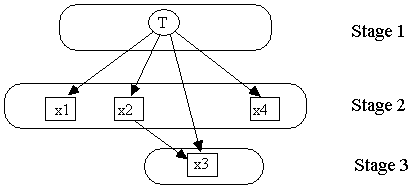
The program's method of generating pseudo-random samples follows the causal structure that produces the joint distribution. This procedure, produces raw sample data one sample unit at a time. For each unit in the sample, it first pseudo-randomly produces a value for each of the exogenous variables, and then a value for each of the variables all of whose parents are exogenous, and so on, until all variables have values. Every iteration handles a tier of variables, where each member of the tier cannot be calculated until all variables in previous tiers are known. The first tier is always the exogenous variables. For example, in generating data for the model in Fig. 13.1, the calculation would proceed in three stages (Fig. 13.5).

Fig. 13.5
The method depends on the factorization of the distribution represented by a Bayesian network. If we are given the joint distribution in factorized form, then we can produce a pseudo-random sample value for each variable whose parents are known. In a Bayesian network, the variables are all discrete, and we simply give the distribution directly. For example, supposing that each variable in the our example from Fig. 13.1 is a binary variable with values in {0,1}, one distribution for this structure is:
p(T = 0) = .4
p(T = 1) = .6
p(x1 = 0|T = 1) = .5 p(x2 = 0|T = 0) = .34 p(x4 = 0|T = 0) = .3
p(x1 = 1|T = 1) = .4 p(x2 = 1|T = 0) = .66 p(x4 =1|T = 0) = .7
p(x1 = 0|T = 0) = .1 p(x2 = 0|T = 1) = .41 p(x4 = 0|T=1) =.25
p(x1 = 1|T = 0) = .1 p(x2 = 1|T = 1) = .61 p(x4 = 1|T =1) =.75
p(x3 = 0|T = 0, x2 = 0) = .5 p(x3 = 0|T = 1, x2 = 0) = .3
p(x3 = 1|T = 0, x2 = 0) = .5 p(x3 = 1|T = 1, x2 = 0) = .7
p(x3 = 0|T = 0, x2 = 1) = .4 p(x3 = 0|T = 1, x2 = 1) = .55
p(x3 = 1|T = 0, x2 = 1) = .6 p(x3 = 1|T = 1, x2 = 1) = .45
Fig. 13.6
Knowing values for all of a variable x's parents, we can look up the appropriate conditional distribution for x and calculate its value by using a simple pseudo-random number generator that produces a uniform distribution over the range [0,1] and appropriate cutoffs. For example, suppose T = 0 and x2 = 1, then the distribution for x3 in Fig. 13.6 is:
p(x3 = 0|T = 0, x2 = 1) = .4
p(x3 = 1|T = 0, x2 = 1) = .6
To give x3 a value, we produce a pseudo-random number from the uniform interval [0,1]. If the number is less than or equal to .4, we assign x3 the value 0; if not, we assign it 1.
In a linear structural equation model, each variable is the effect of its parents and a unique but unobserved error term. Thus the structural equation model associated with the causal structure in Fig. 13.1 is shown in Fig. 13.7.
T = eT
x1 = aT + e1
x2 = bT + e2
x3 = cT + dx2 + e3
x4 = eT + e4
Fig. 13.7
The pair <q,D(e)> is sufficient to characterize the joint distribution for this model, where q is a vector of the linear coefficients and D(e) is a joint distribution on the exogenous variables which are just the independent error terms. Because each variable is simply a linear function of its parents, <q,D(e)> is also sufficient for producing simulated data. In this case, each variable is equal to its error term plus a linear combination of its parents. If the program pseudo-randomly produces a sample value for the error terms, the rest is determined by the linear coefficients.
13.6 Finding Error Probabilities for Search Procedures
One purpose of the Monte Carlo procedure is to enable users to explore the reliability of the model search procedures applied to the investigator's particular problems. When a search procedure yields a model M from a sample, we can ask for the probability that, were the model M true, the procedure would not find some feature of interest of M on samples of that size. The feature of interest could be the presence or absence of a particular adjacency, the presence or absence of a particular oriented edge, the entire pattern, etc. Similarly, we can ask for the probability that were some interesting alternative M' true the search procedure would fail to find some feature of interest of M' on samples of that size. Especially in small samples, the significance levels and powers of the tests used in deciding conditional independence may not be reliable indicators of the probabilities of these types of errors in the search procedure.
Error probabilities for the search procedures in TETRAD II are nearly impossible to obtain analytically, and we recommend that Monte Carlo methods be used instead. When a procedure yields M from a sample of size n, estimate M and use the estimated model to generate a number of samples of size n, run the search procedure on each and calculate the frequency with which the feature of interest of M is incorrect in the output. For plausible or interesting alternative models M', use M' to generate a number of samples of size n, run the search procedure on each and calculate the frequency with which the feature of interest of M' is correct in the output. We give examples of such procedures here.
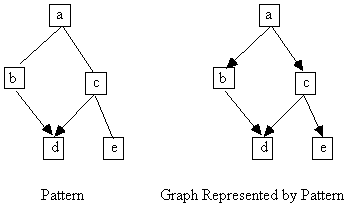
We gave some data to Build, and under the assumption of causal sufficiency, it output the pattern in Fig. 13.8. From among the graphs represented by the pattern, we arbitrarily chose the one shown in Fig. 13.8. The feature of interest in this case is the adjacency of variables b and d.

Fig. 13.8
Using the STATwriter module with the graph shown in Fig. 13.8 and our original data, we formed an input file to the EQS program. Let model M be the estimated model given in the output of EQS. We then generated 50 data sets from M using the Makemod and Monte modules, at each of the sample sizes 100, 500, 1000, and 5000. We ran each of the data sets through Build under the assumption of causal sufficiency with a significance level of .05, and calculated in what percentage of cases the output of Build failed to contain an adjacency between b and d. In this case, because the coefficient corresponding to the edge between b and d is rather large, Build never failed to make them adjacent in any of its output at any of the sample sizes.
Next we constructed several alternatives to M. Model 1 was constructed by adding an edge from a to e to model M, with a coefficient of .1. (The easiest way to consruct a file that represents Model 1 and is readable by TETRAD II is to edit the file produced by the Makemod module for model M.) In this case, the feature of interest is the adjacency of a and e. We then generated 50 data sets from M' using the Monte module at each of the sample sizes 100, 500, 1000, and 5000, and ran each of the data sets through Build under the assumption of causal sufficiency with a significance level of .05. We calculated in what percentage of cases the output of Build failed to contain an adjacency between a and e. We repeated this procedure for Model 2, where the coefficient between a and e was .5, and Model 3, where the coefficient was 1. The results are shown in Table 13.1. The output illustrates that at small sample sizes, Build cannot reliably detect weak causal influences. The reliability may be improved by increasing the signficance level for the smaller sample sizes. However, with larger sample sizes, or larger causal influences, Build does reliably detect the causal connection between a and e.
|
Sample size |
||||
|
|
100 |
500 |
1000 |
5000 |
|
Model 1 |
90 |
70 |
54 |
2 |
|
Model 2 |
6 |
0 |
0 |
0 |
|
Model 3 |
0 |
0 |
0 |
0 |
Table 13.1
We also formed alternative Models 4, 5, and 6, which added to M an edge between d and e with corresponding coefficients .1, .5, and 1.0 respectively. We repeated the process described in the paragaragph above with these 3 alternatives. The results are shown in Table 13.2. In this case, Build requires much larger sample sizes before it becomes reliable. Moreover, when the coefficient between d and e is increased to .5 from .1, the procedure becomes less reliable, not more reliable. This is because the value of .5 is close to a region where faithfulness is violated. (In this case, the partial correlation of d and e given b is very close to zero when the coefficient between d and e is close to .5.) The size of the regions where the probability of error is large because the coefficient is close to a violation of faithfulness, decrease as the sample size increases. In this case, the output of Build may be more reliable for coefficients that lie between .1 and .5 than at either of the endpoints, and it is worthwhile to test the reliability of Build at intermediate values.
|
Sample size |
||||
|
|
100 |
500 |
1000 |
5000 |
|
Model 4 |
100 |
86 |
62 |
0 |
|
Model 5 |
100 |
96 |
78 |
28 |
|
Model 6 |
54 |
4 |
0 |
0 |
Table 13.2