Statistical
Tests';
The Build, Purify, MIMbuild,
and Search modules perform statistical hypothesis tests in order to make
decisions that serve as input for their respective algorithms. In this section we describe these tests and
the distributional assumptions they require.
The Build module uses decisions about (conditional)
independence relations to construct an equivalence class of causal structures.
If the distributional assumptions we discuss below and thus the statistical
tests that accompany them do not seem reasonable for a particular data set you
wish to analyze, then decisions about (conditional) independence can be entered
directly as input to Build. You may use
your own statistical package or whatever means you see fit to make decisions
about (conditional) independence.
A.1 Structural Equation Models
The joint distribution among the nonerror variables V in a recursive structural equation
model (RSEM) is determined by the triple <G, D(e), f>, where G is the causal graph over V, D(e) is the joint distribution among the error terms, and f the linear coefficients that correspond to
each arrow in the path diagram.
Tests for Vanishing
(Partial) Correlation
Under the assumption of multivariate normality, tests for
vanishing (partial) correlation are also tests for (conditional)
independence. That is, rxy.C = 0 Û x || y | C.[1] To test for rxy.C
= 0, TETRAD II uses Fisher's z:

where rx,y.C
= population partial correlation of x and y given C, n is the sample size,
and |C| equals the number of
variables in C. If x, y, and C are normally distributed and rx,y.C
denotes the sample partial correlation of x and y given C, the distribution of z(rx,y.C,n)
- z(rx,y.C,n) is standard normal .;(Anderson,
1984).
Tests for Vanishing Tetrad
Differences
A tetrad difference tijkl = ri,j rk,l - ri,k rj,l. If t vanishes in the population, then t's sample distribution is asymptotically
normal with mean 0 and variance given by Bollen (1990, 1993) in terms of the
fourth moments of the observables. For the case of normally distributed
variables the fourth moments specialize to functions of the covariances, so the
asymptotic variance of a tetrad difference simplifies to a function only of the
covariances. TETRAD II assumes multivariate normal data and uses the .;Wishart
(1928) hypothesis test for a vanishing tetrad difference.
If n is the sample size, then Wishart showed that the sample
tetrad difference tacdb has
(asymptotic) mean tacdb and standard deviation:
SD = ((n+1)/ ((n-1) * (n-2)) * (ra,a * rb,b - ra,b * ra,b) *
(rc,c * rd,d - rc,d * rc,d)) - ((ra,a*d1 - ra,b*d2 + ra,c*d3 - ra,d*d4)/(n - 2))
where
d1 = rb,b * (rc,c * rd,d - rd,c * rd,c) - rb,c * (rc,b * rd,d - rd,c * rd,b) +
rb,d
* (rc,b
* rd,c
- rc,c
* rd,b);
d2 = rb,a * (rc,c * rd,d - rd,c * rd,c) - rb,c * (rc,a * rd,d - rd,c * rd,a) +
rb,d
* (rc,a
* rd,c
- rc,c
* rd,a);
d3 = rb,a * (rc,b * rd,d - rd,c * rd,b) - rb,b * (rc,a * rd,d - rd,c * rd,a) +
rb,d
* (rc,a
* rd,b
- rc,b
* rd,a);
d4 = rb,a * (rc,b * rd,c - rc,c * rd,b) -
rb,b * (rc,a * rd,c - rc,c * rd,a) +
rb,c
* (rc,a
* rd,b
- rc,b
* rd,a);
We calculate SD by substiuting ri,j for ri,j.
The Purify and MIMbuild modules require simultaneous tests
of vanishing tetrad differences. .;Bollen
(1990, 1993) generalized his distribution free test statistic for single tetrad
differences to a simultaneous test that asymptotically approximates a
chi-square variate with degrees of freedom
equal to the number of independent tetrad differences simultaneously
examined. Again, this test is computationally intensive and is not implemented
in TETRAD II, which instead uses the Bonferroni adjustment, also suggested to
us by Bollen (1990). To test the hypothesis that a set of tetrad differences t vanish simultaneously, TETRAD II
requires that each t Î t pass
the Wishart test at a critical level of a/n,
where n = |t|, and a is the user-set significance level.
A.2 Bayesian Networks
When the variables are
discrete valued it is often unrealistic to assume linearity, especially when
the variables are categorical and not even ordinal, for example, gender. TETRAD
II tests for (conditional) independence in multinomial distributions by using
the G2 test for (conditional)
independence in contingency tables given in .;Bishop,
.;Feinberg,
and .;Holland
(1975).
For simplicity consider two variables y1 and y2.
If y1 can take on any of n values,
and if y2 can take on any of m
values, then we form a matrix with n x m cells. The count in a particular cell,
xij, is the value of a random
variable obtained from sampling N units from a multinomial distribution. Let xi+ denote the sum of the counts in all
cells in which the first variable has the value i, and similarly let x+j denote the sum of the counts in all
cells in which the second variable has the value j. On the hypothesis that the
first and second variables are independent, the expected value of the random
variable xij is:

Analogously, we can compute the expected values of cells on
any hypothesis of conditional independence from appropriate marginals. For
example, on the hypothesis that the first variable is independent of the second
conditional on the third, the expected value of the cell xijk is

If there are more than three variables this formula applies
to the expected value of the marginal count of the i, j, k values of the first
three variables, obtained by summing over all other variables. A test of such
an independence hypothesis is:

where Observed is the observed cell count, expected is the
expected cell count, and the summation is over cells. Asymptotically, G2 has a c2 distribution with appropriate degrees
of freedom. TETRAD II calculates the degrees of freedom for a test of the
independence of a and b conditional on C
in the following way. Let Cat(x) be the number of categories of the variable x,
and n be the number of variables in C.
Then the number of degrees of freedom (df) in the test is:

We assume that there are no structural zeroes. As a
heuristic, for each cell of the distribution that has an expected cell count
equal to zero, we reduce the number of degrees of freedom by one.[2]
Because the number of cells grows exponentially with the
number of variables, it is easy to construct cases with far more cells than
there are data points. In that event most cells in the full joint distribution
will be empty, and even nonempty cells may have only small counts. Indeed, it
can readily happen that some of the marginal totals are zero and in these cases
the number of degrees of freedom must be reduced in the test. In testing the
conditional independence of two variables given a set of other variables, if
the sample size is less than 10 times the number of cells to be fitted we
assume the variables are conditionally dependent.
Appendix B
The PC Algorithm';
The Build module uses two algorithms to construct, from
independence and conditional independence data, the class of causal graphs that
entail the same set of (conditional) independence relations over the measured
variables. The PC algorithm is used on
the (conditional) independence relations for a set of variables V assumed to be causally sufficient and
assumed to have an acyclic causal graph that is Markov and Faithful for the
population distribution over V. The
FCI algorithm is used on the (conditional) independence relations for a set of
variables V Í L such that L is causally sufficient and assumed to
have a causal graph that is Markov and Faithful for the population distribution
over V. In chapter 5 we explain the difference in the output of
each. Here we present and explain the
PC algorithm. The more complex FCI algorithm is documented in Causation,
Prediction, and Search, chapter 6.
Let Adjacencies(C,a)
be the set of vertices adjacent to a in a graph C. (In the algorithm, the graph
C is continually updated, so Adjacencies(C,a)
is constantly changing as the algorithm progresses.)
PC Algorithm (Build with causal
sufficiency):
A. Form the
complete undirected graph C on the vertex set V.
B.
n = 0.
repeat
repeat
select an ordered pair of
variables x and y that are adjacent in C such that Adjacencies(C,x)\{y} has cardinality greater than or equal to n,
and a subset S of Adjacencies(C,x)\{y} of cardinality n,
and if x and y are independent given S
delete edge x - y from C and record S
in Sepset(x,y) and Sepset(y,x);
until all ordered pairs of
adjacent variables x and y such that Adjacencies(C,x)\{y}
has cardinality greater than or equal to n and all subsets S of Adjacencies(C,x)\{y}
of cardinality n have been tested for independence;
n = n + 1;
until for each ordered pair of
adjacent vertices x, y, Adjacencies(C,x)\{y}
is of cardinality less than n.
C. For each triple of vertices x,
y, z such that the pair x, y and the pair y, z are each adjacent in C but the
pair x, z are not adjacent in C, orient x - y - z as x ® y ¬ z if and only if y
is not in Sepset(x,z).
D. repeat
1. If x ® y, y and z are adjacent, x and z are not adjacent, and there
is no arrowhead at y, then orient y - z as y ®
z.
2. If there is a directed path from
x to y, and an edge between x and y, then orient x - y as x ® y.
until no more edges can be oriented.
Step 2 of part D has not been implemented in the TETRAD II
program. Although it theoretically enables more edges to be oriented, and
avoids the possibility of cycles, we have found in practice that it decreases
the reliability of the algorithm.
Recall the Markov Equivalence
Theorem:
Markov Equivalence Theorem: Two acyclic causal graphs
over the same variables imply the same independence constraints by the Markov
condition if and only if (a) they have the same adjacencies, and (b) they have
the same unshielded colliders.
Because any two causal graphs
that differ on a single adjacency are distinguishable, the PC algorithm first
identifies the adjacencies and then orients them.

Fig. B.1
Adjacency
The PC algorithm begins with every pair of variables
adjacent and then removes adjacencies upon finding (conditional) independence
relations in the data. By the Markov condition, if x and y are not adjacent,
then x and y are independent conditional on the parents of x or on the parents
of y, or on both. We don't know which variables are the parents of x or the
parents of y. But we do know at each stage of the algorithm that the parents of
x are included in the set of vertices adjacent to x, and the parents of y are
included in the set of vertices adjacent to y. At the nth stage of the algorithm, if there is
still an edge between a and b in the graph constructed thus far, then the
algorithm tests whether the edge should be removed by testing whether a and b
are independent conditional on any subset of the variables adjacent to a (and
that does not include b) of size n, or independent conditional on any subset of
the variables adjacent to b (and that does not include a) of size n. It removes
the edge between a and b if and only if it finds such a conditional
independence.
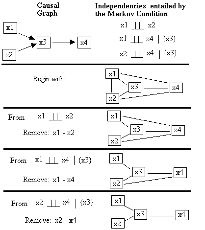
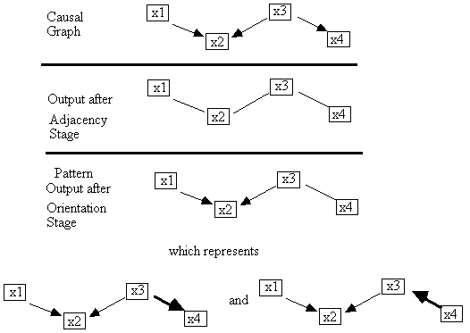
For example, in Fig. B.2 we show the progression of the
adjacency stage of PC on the independence relations implied by the causal graph
shown at the top. Beginning with every
pair adjacent, which we represent with an undirected edge, the algorithm first
considers independencies in which the conditioning set is empty. From the fact that x1 || x2, the algorithm
eliminates the x1-x2 adjacency and proceeds.

Fig. B.2
After the x1-x2 and the x1-x4 adjacencies have been removed,
testing the x2-x4 adjacency requires only that x2 and x4 be conditioned on the
set: {x3}, because it is the only member of either Adjacencies(C,x2)\{x4} or Adjacencies(C,x4)\{x2}.
In larger graphs, this efficiency in the conditioning sets PC need consider
translates into enormous speed-up.
In practice, of course, adjacencies will be removed
appropriately so long as the statistical decision to accept an independence
relation is made correctly. Accordingly, in Build's output, TETRAD II prints
out statistical information about each of the decisions that led to the removal
of an adjacency, or edge. For example,
part of the output produced by the Build module on data pseudo-randomly
generated from a linear model with the structure at the top of Fig. B-2 is as
follows.
List of vanishing
(partial) correlations that made
TETRAD remove edges from
the graph.
Corr. : Sample (Partial)
Correlation
Prob. : Probability that
the absolute value of the sample
(partial) correlation exceeds the observed value,
on the assumption of zero (partial) correlation in
the population, assuming a multinormal
distribution.
Edge (Partial)
Removed Correlation Corr. Prob.
------- ----------- ----- -----
x1 -- x2 rho(x1 x2) 0.0250
0.2639
x2 -- x4 rho(x2 x4 . x3) 0.0286 0.1999
x1 -- x4 rho(x1 x4 . x3) -0.0300 0.1799
Fig. B-3
TETRAD II accepts an independence relation as holding in the
population in case it cannot reject it at the significance level chosen by the
user. The default, that was used here, is .05.
Orientation
The Markov Equivalence
theorem states that two models with identical adjacencies can be distinguished
if they have different sets of unshielded colliders. Accordingly, PC searches
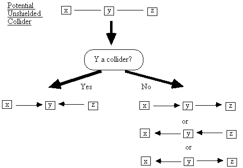
for triples of variables x, y, and z such that x and y are adjacent, y and z
are adjacent, but x and z are not (Fig. B.4).
We call such triples potential
unshielded colliders.

Fig. B-4: Potential Unshielded
Collider
Because x and z are not adjacent, there is some set S Ì
V such that x and z are independent
conditional on S, that is, x || z | S. Assuming
faithfulness, if y is a noncollider on the x -
y - z path, then y is in every
set S that makes x and z
independent. If y is a collider on the x - y
- z path, then x and z will be dependent conditional on every set that
contains y. Hence, for every set S
such that x || z | S,
y is a collider on the x - y - z path if and only if y Ï S.
The set S corresponds to the set
Sepset(x,z) in the statement of the
algorithm above.
If y is a collider on the x -
y - z path, and we have assumed
that our system is causally sufficient, then we can orient x-y-z as x ® y ¬ z. If y is not a collider, however, then three
orientations are possible (Fig. B.5).

Fig. B.5
The PC algorithm's orientation stage begins with the
unoriented adjacencies that the adjacency stage outputs. It then proceeds through all potential
unshielded collider triples and orients any that are colliders (step C). It then revisits these triples and looks for
any that have been partially oriented toward a collider, for example, Fig. B.6,
that is, one edge is directed toward the vertex common to both adjacencies and
the other edge is unoriented (step D.1).

Fig. B.6
One way these triples arise is when in the causal structure
that generated the data there is some w such that y is a collider on the x - y - w
path, but not a collider on the x - y - z path, for example, Fig. B.7.

Fig. B.7
After every potential unshielded collider has been
considered, then one that is partially oriented as in Fig. B.7 can arise only
if y is a non-collider on the x - y - z path, because otherwise it would have
been fully oriented when it was originally considered. But now the y -
z adjacency cannot be y ¬ z,
because that would make y a collider on any path that contains x-y-z,
so we orient
it away from a collider as y ® z.
The PC algorithm cycles through all potential unshielded
colliders that are not fully oriented and applies the away from a collider test
until it has traversed the set without changing anything. Using the same example as we did in the
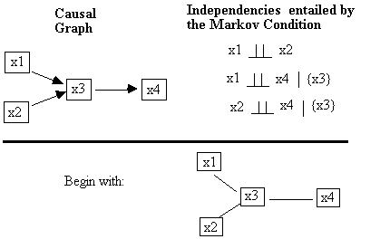
adjacency stage, we trace the execution of the orientation phase.
PC: Orientation Phase

Fig. B.8
There are three potential unshielded colliders in this
structure (Fig. B.9).

Fig. B.9
In the first, we determine whether x3 is a collider on the
x1-x3-x2 path by looking at the set that made x1 and x2 independent. In this case x1 and x2 are independent
unconditionally, so x3 is not in the set and therefore x3 must be a
collider.

Fig. B.10
In potential unshielded collider number 2, x3 is in the set
that separated x1 and x4, so it is not a collider on the x1-x3-x4 path. In potential unshielded collider number 3,
x3 is in the set that separated x2 and x4, so it is not a collider on the
x2-x3-x4 path. So after the first cycle through the potential unshielded
colliders, the pattern has the structure shown in Fig. B.10.
Upon visiting the updated potential unshielded colliders
again, PC will find the updated three we show in Fig. B.11. It searches for ones that are partially
oriented toward a collider, for example, numbers 2 and 3.

Fig. B.11
Both of these require that the x3-x4 adjacency must be
oriented as x3®x4, so the final PC
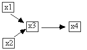
output for this case is Fig. B.12, which is precisely the causal structure that
generated the data.

Fig. B.12: Final PC Output
In this case the algorithm output a pattern that represents
a single graph, but of course the output is often less informative. For example
in Fig. B.13 we show the algorithm's progression on the independence relations
implied by the graph at the top.

Fig. B.13
In this case the algorithm cannot orient the x3 - x4 adjacency, because orienting it does
not change the set of unshielded colliders. When causal sufficiency is assumed,
PCs output is a pattern that represents all the causal graphs that can be
generated by any orientation of the unoriented adjacencies that do not create
an additional unshielded collider or a cycle.
In this case there are only two such graphs. In general the number of distinct causal graphs represented by a
pattern is bounded above by 2n,
where n is the number of unoriented adjacencies. 2n is only an upper bound because
pairs of unoriented adjacencies that share a vertex, for example, x - y - z,
cannot be oriented as x ® y ¬ z, so instead of 22 = 4 possible orientations there are
only 3.
PC and Temporal Knoweldge
If G is a Markov and Faithful
causal graph for probability distribution P and V a set of causally sufficient variables for G, and y is not an
ancestor of x, then x and y are not adjacent in G if and only if they are
independent conditional on y's parents in G. This entails that in all cases x
and y are not adjacent if and only if they are independent conditional on
either y's parents or on x's.
At intermediate stages of the PC
algorithm without temporal knowledge, x might be an ancestor of y or y of x,
and all of the variables still adjacent to x might be x's parents and all of
the variables still adjacent to y might be y's parents. Thus the PC algorithm without temporal
knowledge tests for adjacency between x and y by conditioning on every subset
of the neighbors of x and every subset of the neighbors of y, that is, every
subset of Adjacencies(C,x)\{y} and
every subset of Adjacencies(C,y)\{x}.
When information about the time order is known, then many of these conditioning
sets can be eliminated. For example, if x is known to be before y, then only
subsets of the neighbors of y need be conditioned on (i.e., subsets of Adjacencies(C,y)\{x}).
If some of the neighbors of y are
known to be subsequent to y, then they cannot be parents of y and need not be
conditioned on either. That is, if S
= {v | v is not known to be later than y} then T = S Ç Adjacencies(C,y)\{x})
is a set such that x and y are adjacent if and only if they are dependent
conditional on every subset of T.
See section 5.7.2 for how to enter
temporal knowledge to the Build module.
Appendix C
Purify';
C.1 The Algorithms in Purify
Purify uses tetrad
constraints to locate and discard indicators that are impure in the true model.
In a directed acyclic graph G with measured variables M and latent variables T,
an indicator xi is a pure indicator of a latent
variable T if it is a direct effect of T and no other variable in T È
M, the cause of no variable in T È
M, and for every other error
variable ej (j in T È M),
ei
and ej
are uncorrelated. xi
is an almost pure indicator
of T if xi is a direct effect
of T and the graph entails that xi is
independent of every other variable in T
È M
conditional on T.

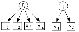
Fig. C.1
For all paramaterizations of
a model in which x1, x2, x3,
and x4 are almost pure
indicators of Ti, and y1 and y2
are almost pure indicators of Tj
(e.g., Fig. C.1):
rx1,x2 * rx3,x4 = rx1,x3 * rx2,x4 = rx1,x4 * rx2,x3 [1]
rx1,x2 * rx3,y1 = rx1,x3 * rx2,y1 = rx1,y1 * rx2,x3 [2]
Tetrad equations in which all four variables measure the
same latent, as in Equation 1, are called 4x0
tetrads. Tetrad equations in which
three indicators measure one latent and the remaining indicator measures
another, as in Equation 2, are called 3x1 tetrads. In the first, or
Intra-Construct stage, Purify considers only 4x0 tetrads among the indicators
for each latent variable with four indicators or more. If there are exactly four indicators, it
cannot prune any, but it will give information about how many of the three
tetrads implied fail the Bonferroni test (described in Appendix A.)
If there are more
than four indicators, then Purify calculates a heuristic "score" for
each indicator, pruning the indicator that has the lowest score, and then
iterating until a set has four indicators or no tetrad equation fails the
Bonferroni test. The
"score" is
calculated as follows. If t is a tetrad
difference, let P(t) be the probability that a sample value of
the tetrad difference exceeds the observed value of the tetrad difference,
given that the population tetrad difference is zero. Thus if the significance level is a,
a tetrad difference t is judged to be
equal to zero in the population if P(t)
≥ a. Let Implied(Gx) be the set of 4x0 tetrad differences
in a measurement model G that involves the indicator x. For each t Î Implied(Gx), t
= 0 if x is almost pure in
G. For a given data set, let Held be
the set of tetrad differences that are judged to be equal to zero in the
population, and ~Held be the set of tetrad differences that are judged not to be
equal to zero in the population. Once
the associated probabilities of all of the tetrad differences have been
calculated, the score of an indicator x in a pure measurement model G can be
calculated in the following way:

For each equation that is judged to hold, the score is
increased by an amount proportional to P(t),
and for each equation that is judged not to hold, the score is decremented by
an amount proportional to how close P(t)
is to 0. The weight
parameter controls
the relative importance attached to explaining true equations as opposed to
failing to imply false ones.
After using 4x0 tetrads to prune indicators, Purify turns to
the Cross-Construct stage, which involves 3x1 tetrads. In each stage Purify
follows a procedure similar to the one described before, with the only
difference being the set of tetrads considered. In the 3x1 stage, Implied(Gx)
is now the set of every 3x1 tetrad difference in a measurement model G that
involves the indicator x. Again, for each t
Î Implied(Gx), t = 0 if x is almost pure in G, and the
score for x is calculated the same way.
C.2 Purify's Theoretical Reliability
Let G be a causal graph over T È V È C. G is a latent variable model if it is a
recursive linear structural equation model and:
1. T is a causally sufficient set of latent variables.
2. V is a set of measured variables such that each v Î V
is the direct effect of at least one member of T and v is the cause of no member of T È C.
3. C is a set of latent variables disjoint from T such that each member
of C is either a common cause of some T and v, or
is a common cause of vi, vj.
4. V can be partitioned into V(Ti) such that for every Ti Î
T, |V(Ti)| > 2, and
for every v Î V(Ti), v measures
Ti, i.e., v is a direct effect
of Ti.
Purify Reliability Theorem:[3] If G is a latent variable model that implies
every 3x1 tetrad equation among V
for every parameterization of G, then for every Ti Î T, and every v Î V(Ti) such that |V(Ti)| > 2, v
is almost pure.
Appendix D
MIMbuild';
D.1 The Algorithms in MIMbuild
MIMbuild begins with an almost pure measurement model and
attempts to find pairs of latent variables that are independent or
conditionally independent given another latent. It then constructs the set of structural models that entail such
independence relations for all possible parameterizations. Such constraints on the latent variables can
be tested from only the marginal covariance matrix involving the measured
variables, provided that the measurement model is almost pure.
0-order Tests

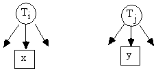
Fig. D.1: rx,y
= 0 Û rTi,Tj = 0
If x is an almost pure indicator of Ti and y is an almost pure indicator of Tj (Fig. D.1), then
rx,y
= 0 Û
rTi,Tj = 0
If x and y are almost pure, then we say that rx,y
= 0 is a test for a 0-order
constraint among the latent variables that they measure.
Because each latent has several indicators, MIMbuild
performs a hypothesis test on rTi,Tj = 0 by simultanteously testing rx,y
= 0 for every x that is an almost pure measure of Ti and every y that is an almost pure measure of Tj. The simultaneous tests are performed
with a Bonferroni adjusted significance level (described in Appendix A).
1st-order Tests

Fig. D.2
If the distribution is faithful to the true causal graph, x
is an almost pure indicator of Ti,
y is an almost pure indicator of Tj,
and z1 and z2 are almost pure indicators of Tk (Fig. D.2), then:[4]
rTi,Tj.Tk = 0 Û rx,y * rz1,z2
= rx,z1 * ry,z2 = rx,z2
* ry,z1
We say that rx,y * rz1,z2 =
rx,z1 * ry,z2 is a test for a 1st-order
constraint among the latent variables. Again, because each latent variable has
several indicators, there will be several redundant tests of a hypothesis rTi,Tj.Tk
= 0. Again MIMbuild performs each such
test with a Bonferroni
adjusted significance level (described in Appendix A.) After determining the 0
and 1st-order constraints on the latent variables in the structural model,
MIMbuild uses the PC algorithm (with its input limited to 0 and 1st order
independence relations) to determine its output.
Question Marks
Some adjacencies cannot be eliminated with only 0 or
1st-order tests.[5] As a result MIMbuild's output will sometimes
contain adjacencies that could have been eliminated with higher order tests.[6] Because of this MIMbuild offers the option
of putting question marks on adjacencies that it cannot be certain are present
in the true model, even if all of the modelling assumptions have been
satisfied. These adjacencies are marked with a "?". On the other hand
there are other adjacencies that MIMbuild can be certain are present in the
true model,when all of the modelling assumptions have been satisfied. These
adjacencies are not marked with a "?".
For any two latents Ti
and Tj in the pattern P that MIMbuild has constructed so far, let P be the set of all undirected paths
between Ti and Tj
that don't include the Ti-Ti
edge. If Ti and Tj
are adjacent in P, then MIMbuild marks
the edge between Ti and Tj with a "?" unless either
1. no paths
are in P, or
2. every
path in P contains a collider, or
3. there
exists a vertex z such that z is a noncollider on every path in P, or
4. every
path in P contains the same subpath
<A,B,C>.
Assuming causal sufficiency among the latents guarantees
that these conditions are correct in the following sense. If G is the model
that generated the data, and P is the
pattern output by MIMbuild, then every edge in P
without a question mark exists in G.
D.2 MIMbuild's Theoretical Reliability
Given all of its assumptions, how reliable is MIMbuild's
output on population data? We assume:
1. G is a recursive linear
structural model with an almost pure measurement model M for a causally
sufficient set of latent variables T.
2. MIMbuild is given M or a
submodel of M with at least three indicators per latent as its input
measurement model.
3. MIMbuild correctly identifies
all and only the set of 0 and 1st-order contraints among the latent variables
implied for every parameterization of G.
A trek between a
pair of distinct variables a and b is either a directed path from a to b, a
directed path from b to a, or a pair of directed paths from some other variable
c to a and b respectively, such that the paths intersect only at c.
Under these assumptions, if P
is the pattern output by the MIMBuild Algorithm then:
A-1. If Ti
and Tj are not adjacent
in P, then they are not adjacent in G.
A-2. If Ti
and Tj are adjacent in P and the edge is not labeled with a
"?", then Ti and Tj
are adjacent in G.
O-1. If Ti
® Tj is in P, then
every trek in G between Ti and Tj
is into Tj.
O-2. If Ti ® Tj is in P
and the edge between Ti and Tj
is not labeled with a "?", then Ti ® Tj is in G.
In fact only A-2 and O-2 depend on causal sufficiency among
the latents. Without assuming causal
sufficiency, MIMbuild's output is still reliable in the sense of A1 and
O1. Both are negative sorts of
knowledge, and can be useful in eliminating theoretical hypotheses of interest.
A-1 allows us to conclude that if there is no edge between Ti and Tj
in P, then whatever the causal
connection between Ti and Tj it is mediated by other latents in our
model. O-1 allows us to conclude that
if there is a directed edge Ti
® Tj
in P, then there is no causal path of any sort from Tj to Ti.

![]()
![]()
![]()


